Neural Network Architectures

CSI 4106 - Fall 2026

Marcel Turcotte

Version: Sep 13, 2026 16:21

Preamble

Message of the Day

Learning outcomes

By the end of this lecture, you should be able to:

  • Explain how local connectivity and parameter sharing give convolutional networks an inductive bias and reduce parameter counts.
  • Compute and trace the forward pass of a 1D convolutional layer with multiple input channels, kernels, biases, and activations.
  • Determine how kernel size, padding, stride, and pooling affect output shape, boundary behaviour, and retained positional information.
  • Explain how stacked layers compose features, enlarge receptive fields, and supply a prediction head.
  • Distinguish translation equivariance from invariance, including the roles of convolution and position aggregation.

Convolutional Neural Network (CNN)

Motivation

“An MLP with just one hidden layer can theoretically model even the most complex functions, provided it has enough neurons. But for complex problems, deep networks have a much higher parameter efficiency than shallow ones: they can model complex functions using exponentially fewer neurons than shallow nets, allowing them to reach much better performance with the same amount of training data.”

Motivation (continued)

  • Consider an RGB image with dimensions \(224 \times 224\), which is relatively small by contemporary benchmarks.
  • The image consists of \(224 \times 224 \times 3 = 150,528\) input features.
  • A neural network with merely a single hidden dense layer would require over 22,658,678,784 (22 billion) parameters, highlighting the computational complexity involved.

Concepts

Our discussion will center around the following key concepts.

  • Inductive bias and topological priors
  • Local connectivity and sparse interactions
  • Parameter sharing and equivariance
  • Hierarchical feature composition
  • Translation equivariance and invariance through position aggregation

Classical image processing

Intuition/2D Historical Context

  • Classical 2D image processing establishes motivation before introducing the underlying methodology.
  • Distinguishes the visual intuition from the matrix operations.

How does a kernel scan an image?

Show code
from pathlib import Path

import numpy as np
import pandas as pd
import matplotlib.pyplot as plt
from matplotlib.colors import Normalize
from matplotlib.patches import Rectangle
from PIL import Image

SAMPLE_RATE = 50

BLUE = "#0072B2"
ORANGE = "#D55E00"
GREEN = "#009E73"
PURPLE = "#CC79A7"
GRAY = "#5B6573"
LIGHT_GRAY = "#D8DCE2"
HIGHLIGHT = "#F0E442"

plt.rcParams.update({
    "axes.spines.top": False,
    "axes.spines.right": False,
    "axes.titleweight": "bold",
    "axes.labelsize": 12,
    "axes.titlesize": 14,
    "font.size": 12,
    "legend.frameon": False,
    "lines.linewidth": 2.2,
})

# A small, long-form extract from the UCI HAR inertial-signal files.
data_path = Path("data/uci_har_prototype.csv")
signals = pd.read_csv(data_path)

walking = (
    signals.loc[signals["activity"] == "walking"]
    .sort_values("sample")
    .reset_index(drop=True)
)
sitting = (
    signals.loc[signals["activity"] == "sitting"]
    .sort_values("sample")
    .reset_index(drop=True)
)

time = walking["sample"].to_numpy() / SAMPLE_RATE
x_walking = walking["x"].to_numpy()


def style_time_axis(ax, *, xlabel=False, ylabel=None, ylim=None):
    """Apply a shared visual style to the signal plots."""
    ax.axhline(0, color=LIGHT_GRAY, linewidth=1, zorder=0)
    ax.grid(axis="x", color=LIGHT_GRAY, linewidth=0.7, alpha=0.55)
    ax.set_xlim(time[0], time[-1])
    if ylim is not None:
        ax.set_ylim(*ylim)
    if ylabel:
        ax.set_ylabel(ylabel)
    if xlabel:
        ax.set_xlabel("time (s)")
    else:
        ax.tick_params(labelbottom=False)
Show cross-correlation code
def cross_correlation2d(X, K):
    """Apply a 2D kernel as written, using valid cross-correlation."""
    output_rows = X.shape[0] - K.shape[0] + 1
    output_cols = X.shape[1] - K.shape[1] + 1
    Y = np.zeros((output_rows, output_cols), dtype=float)

    for i in range(output_rows):
        for j in range(output_cols):
            total = 0.0
            for u in range(K.shape[0]):
                for v in range(K.shape[1]):
                    total += X[i + u, j + v] * K[u, v]
            Y[i, j] = total

    return Y


def draw_number_matrix(ax, values, title, *, cmap="Greys", vmin=None,
                       vmax=None, text_color=None):
    """Display a small matrix with its numerical values."""
    ax.imshow(values, cmap=cmap, vmin=vmin, vmax=vmax)
    rows, cols = values.shape
    norm = Normalize(vmin=np.min(values) if vmin is None else vmin,
                     vmax=np.max(values) if vmax is None else vmax)
    color_map = plt.get_cmap(cmap)
    for i in range(rows):
        for j in range(cols):
            value = 0.0 if np.isclose(values[i, j], 0.0) else values[i, j]
            ax.add_patch(Rectangle(
                (j - 0.5, i - 0.5), 1, 1,
                fill=False, edgecolor="#7A7A7A", linewidth=1.6,
            ))
            if text_color is None:
                red, green, blue, _ = color_map(norm(value))
                luminance = 0.2126 * red + 0.7152 * green + 0.0722 * blue
                cell_text_color = "black" if luminance > 0.52 else "white"
            else:
                cell_text_color = text_color
            ax.text(j, i, f"{value:g}", ha="center", va="center",
                    color=cell_text_color, fontsize=17, fontweight="bold")
    ax.set_xticks([])
    ax.set_yticks([])
    ax.set_title(title, pad=12)


X_image = np.array([
    [255, 255, 255, 255],
    [255,   0,   0, 255],
    [255,   0,   0, 255],
    [255, 255, 255, 255],
], dtype=float)

K_edge = np.array([
    [-1, 1],
    [-1, 1],
], dtype=float)

Y_image = cross_correlation2d(X_image, K_edge)
placement_order = np.arange(1, 10).reshape(3, 3)

fig, axes = plt.subplots(
    1, 3,
    figsize=(11.4, 4.4),
    gridspec_kw={"width_ratios": [1.25, 0.78, 1.0]},
)

draw_number_matrix(
    axes[0], X_image, "Input image $X$", cmap="Greys_r", vmin=0, vmax=255,
)
axes[0].add_patch(Rectangle(
    (-0.5, -0.5), 2, 2,
    facecolor="none", edgecolor=ORANGE, linewidth=4,
))
draw_number_matrix(
    axes[1], K_edge, "Kernel $K$", cmap="RdBu_r", vmin=-1, vmax=1,
)

draw_number_matrix(
    axes[2], placement_order, "Nine valid placements", cmap="Greys",
    vmin=0, vmax=100,
)

fig.tight_layout(w_pad=2.0)
plt.show()
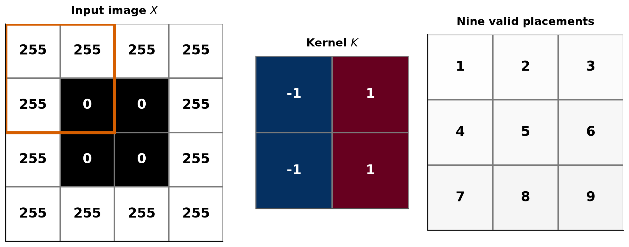
A four-by-four grayscale image of the letter O, a two-by-two edge kernel, and a three-by-three map numbering the nine valid kernel placements.

What does each placement compute?

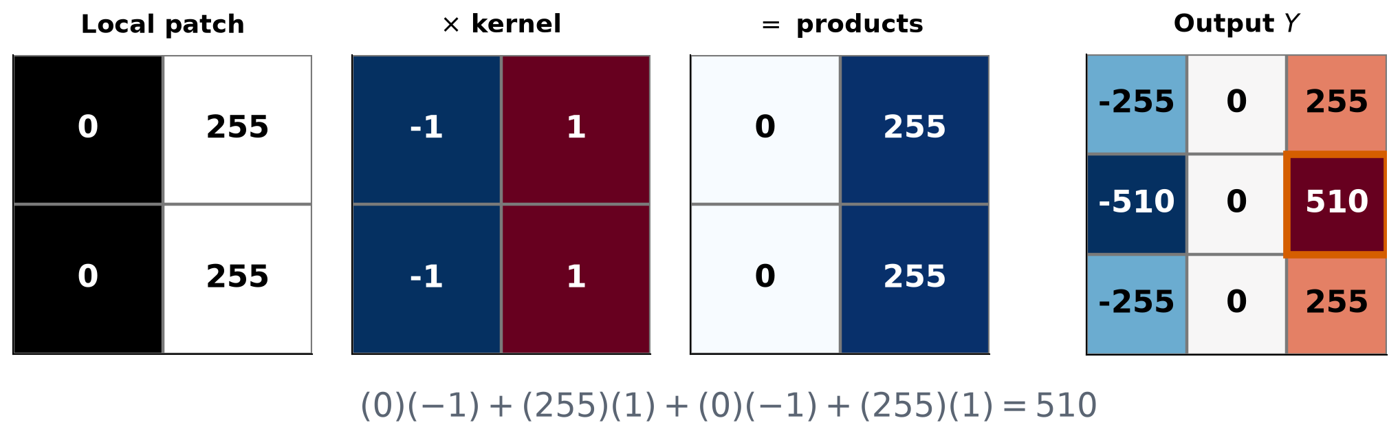
\[ Y[i,j] = \sum_{u=0}^{K_h-1}\sum_{v=0}^{K_w-1} X[i+u,j+v] K[u,v] \]

Show calculation code
i, j = 1, 2
patch = X_image[i:i + K_edge.shape[0], j:j + K_edge.shape[1]]
products = patch * K_edge

fig, axes = plt.subplots(
    1, 4,
    figsize=(11.2, 3.25),
    gridspec_kw={"width_ratios": [0.9, 0.9, 0.9, 1.25]},
)

draw_number_matrix(axes[0], patch, "Local patch", cmap="Greys_r", vmin=0, vmax=255)
draw_number_matrix(axes[1], K_edge, r"$\times$ kernel", cmap="RdBu_r", vmin=-1, vmax=1)
draw_number_matrix(axes[2], products, "$=$ products", cmap="Blues", vmin=0, vmax=255)
draw_number_matrix(axes[3], Y_image, "Output $Y$", cmap="RdBu_r", vmin=-510, vmax=510)
axes[3].add_patch(Rectangle(
    (j - 0.5, i - 0.5), 1, 1,
    facecolor="none", edgecolor=ORANGE, linewidth=4,
))

fig.text(
    0.50, 0.02,
    r"$(0)(-1)+(255)(1)+(0)(-1)+(255)(1)=510$",
    ha="center", fontsize=18, color=GRAY,
)
fig.tight_layout(rect=[0, 0.11, 1, 1], w_pad=1.8)
plt.show()

One image patch and the edge kernel are multiplied element by element, summed to 510, and entered in the corresponding output position.

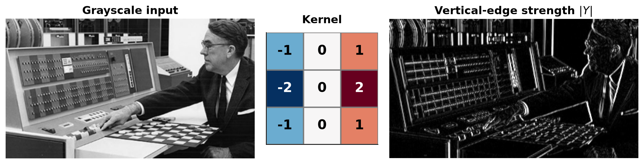
Which kernel reveals vertical edges?

Show edge-detection code
photo_path = Path("images/ibm_704.jpeg")
photo = Image.open(photo_path).convert("L")
photo.thumbnail((360, 360))
photo_gray = np.asarray(photo, dtype=float) / 255.0

K_vertical = np.array([
    [-1, 0, 1],
    [-2, 0, 2],
    [-1, 0, 1],
], dtype=float)

Y_vertical = cross_correlation2d(photo_gray, K_vertical)
vertical_strength = np.abs(Y_vertical)
vertical_limit = np.percentile(vertical_strength, 99)

fig, axes = plt.subplots(
    1, 3,
    figsize=(11.5, 4.4),
    gridspec_kw={"width_ratios": [1.38, 0.62, 1.38]},
)

axes[0].imshow(photo_gray, cmap="gray", vmin=0, vmax=1)
axes[0].set_title("Grayscale input")
axes[0].axis("off")

draw_number_matrix(
    axes[1], K_vertical, "Kernel",
    cmap="RdBu_r", vmin=-2, vmax=2,
)

axes[2].imshow(
    vertical_strength, cmap="gray", vmin=0, vmax=vertical_limit,
)
axes[2].set_title("Vertical-edge strength $|Y|$")
axes[2].axis("off")

fig.tight_layout(w_pad=1.2)
plt.show()

A grayscale photograph, a Sobel kernel that measures changes across columns, and the resulting vertical-edge strength image.

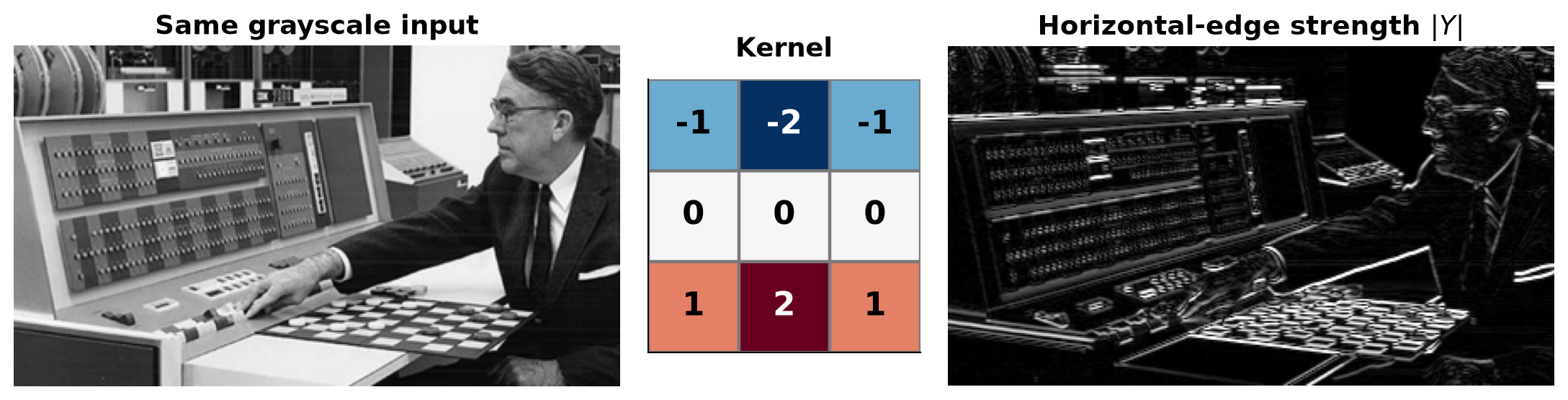
How can we reveal horizontal edges?

Show edge-detection code
K_horizontal = np.array([
    [-1, -2, -1],
    [ 0,  0,  0],
    [ 1,  2,  1],
], dtype=float)

Y_horizontal = cross_correlation2d(photo_gray, K_horizontal)
horizontal_strength = np.abs(Y_horizontal)
horizontal_limit = np.percentile(horizontal_strength, 99)

fig, axes = plt.subplots(
    1, 3,
    figsize=(11.5, 4.4),
    gridspec_kw={"width_ratios": [1.38, 0.62, 1.38]},
)

axes[0].imshow(photo_gray, cmap="gray", vmin=0, vmax=1)
axes[0].set_title("Same grayscale input")
axes[0].axis("off")

draw_number_matrix(
    axes[1], K_horizontal, "Kernel",
    cmap="RdBu_r", vmin=-2, vmax=2,
)

axes[2].imshow(
    horizontal_strength, cmap="gray", vmin=0, vmax=horizontal_limit,
)
axes[2].set_title("Horizontal-edge strength $|Y|$")
axes[2].axis("off")

fig.tight_layout(w_pad=1.2)
plt.show()

The same grayscale photograph, a Sobel kernel that measures changes across rows, and the resulting horizontal-edge strength image.

Central computational idea

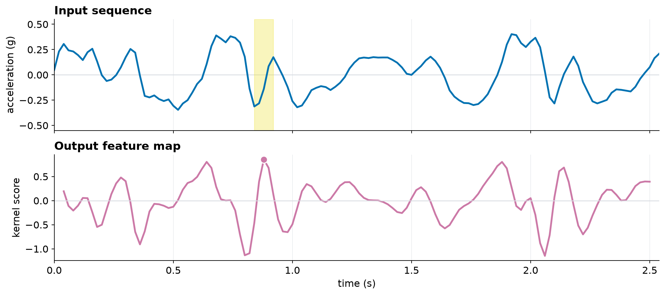
A small set of weights (kernel/filter) is applied to every local neighbourhood, producing a response (feature) map that records where the selected pattern occurs.

Convolution in one dimension

Where do 1D data appear?

What problems have observations arranged along one ordered axis?

\[ x[0],\; x[1],\; x[2],\; \ldots,\; x[L-1] \]

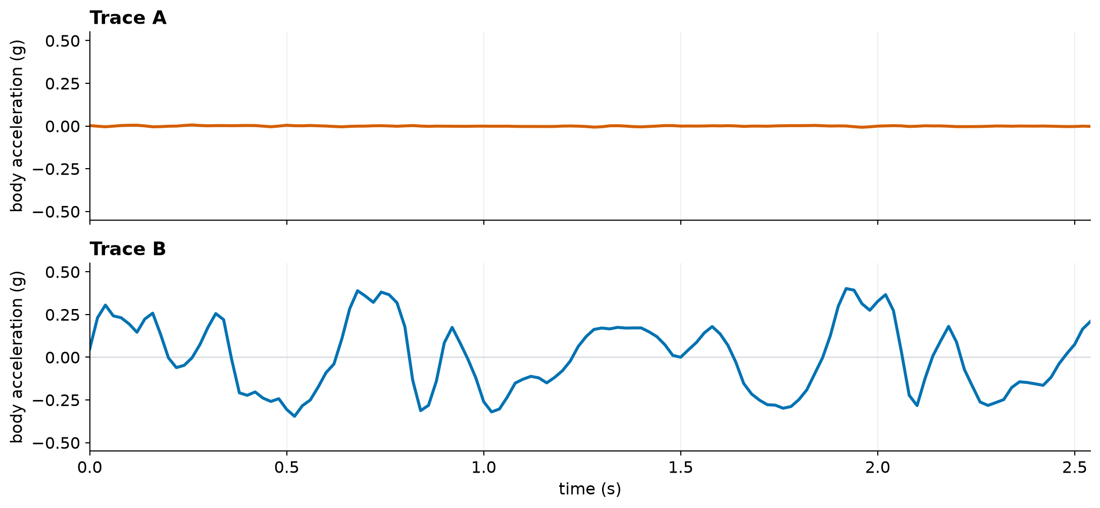
Which trace comes from walking?

Show plotting code
fig, axes = plt.subplots(2, 1, figsize=(11.5, 5.4), sharex=True)

for ax, frame, title, color in [
    (axes[0], sitting, "Trace A", ORANGE),
    (axes[1], walking, "Trace B", BLUE),
]:
    ax.plot(time, frame["x"], color=color)
    ax.set_title(title, loc="left")
    style_time_axis(
        ax,
        xlabel=ax is axes[-1],
        ylabel="body acceleration (g)",
        ylim=(-0.55, 0.55),
    )

fig.tight_layout(h_pad=1.0)
plt.show()

Two aligned body-acceleration traces: a nearly flat sitting signal and a larger oscillating walking signal.

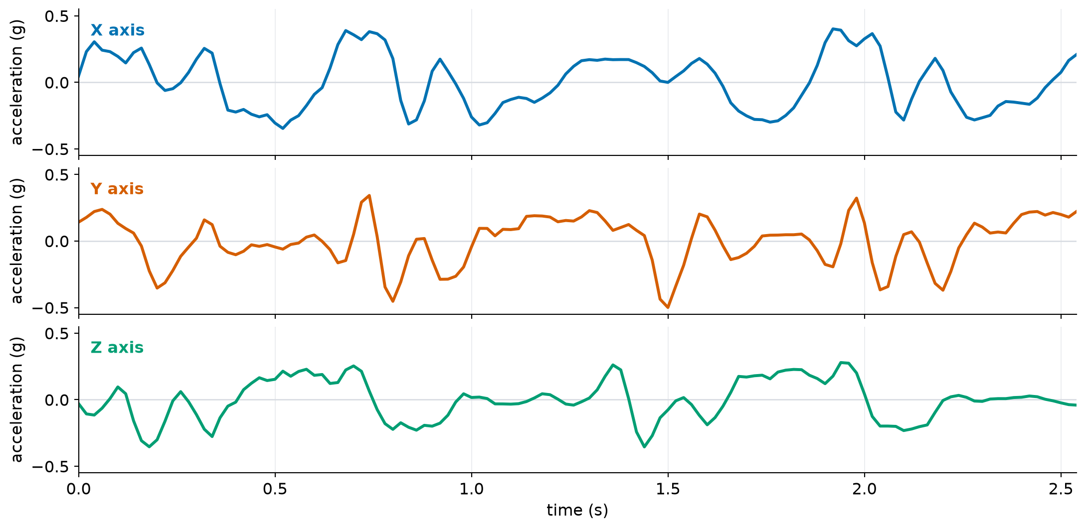
A phone records three sequences

Show plotting code
fig, axes = plt.subplots(3, 1, figsize=(11.5, 5.7), sharex=True)

for ax, channel, color in zip(axes, ["x", "y", "z"], [BLUE, ORANGE, GREEN]):
    ax.plot(time, walking[channel], color=color)
    ax.text(
        0.012,
        0.82,
        f"{channel.upper()} axis",
        transform=ax.transAxes,
        color=color,
        fontweight="bold",
    )
    style_time_axis(
        ax,
        xlabel=ax is axes[-1],
        ylabel="acceleration (g)",
        ylim=(-0.55, 0.55),
    )

fig.tight_layout(h_pad=0.45)
plt.show()

Three aligned walking body-acceleration signals from a phone's X, Y, and Z axes.

A signal is an ordered list of numbers

first_values = pd.DataFrame({
    "index i": walking["sample"].head(8),
    "time (s)": (walking["sample"].head(8) / SAMPLE_RATE).round(2),
    "x[i] (g)": walking["x"].head(8).round(5),
})
print(first_values.to_string(index=False))
 index i  time (s)  x[i] (g)
       0      0.00   0.04796
       1      0.02   0.23134
       2      0.04   0.30507
       3      0.06   0.24206
       4      0.08   0.23098
       5      0.10   0.19504
       6      0.12   0.14604
       7      0.14   0.22359

\[ x[0]=0.04796,\quad x[1]=0.23134,\quad x[2]=0.30507,\quad\ldots \]

What should the model assume?

  • Nearby measurements form meaningful local patterns.
  • A useful pattern may occur at different positions.
  • The same detector should be reused everywhere.

One kernel scores one local contrast

Show plotting code
kernel_up = np.array([-1.0, -1.0, 0.0, 1.0, 1.0])
kernel_down = -kernel_up
K = kernel_up.size

# This window happens to cross zero; the kernel itself compares relative levels.
start = 11
stop = start + K

fig, ax = plt.subplots(figsize=(9.0, 3.4))
ax.plot(time, x_walking, color=BLUE)
ax.axvspan(
    time[start],
    time[stop - 1],
    color=HIGHLIGHT,
    alpha=0.35,
    label="local window",
)
ax.scatter(
    time[start:stop],
    x_walking[start:stop],
    color=BLUE,
    edgecolor="white",
    linewidth=1.2,
    s=58,
    zorder=3,
)
style_time_axis(
    ax,
    xlabel=True,
    ylabel="body acceleration (g)",
    ylim=(-0.55, 0.55),
)
ax.legend(loc="upper right")
fig.tight_layout()
plt.show()

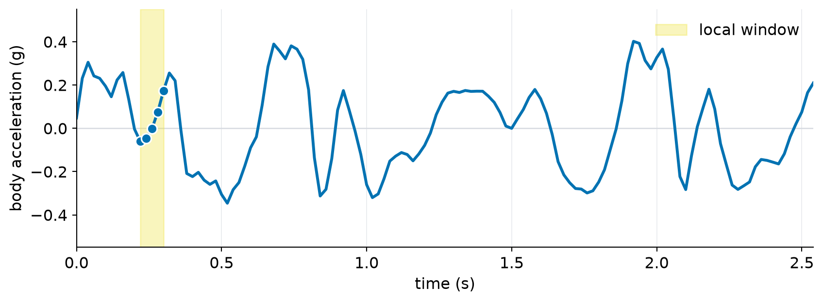
A walking acceleration trace with five adjacent samples highlighted as a local kernel window.

\[ w = [-1,-1,0,1,1], \qquad y[i] = \sum_{j=0}^{K-1} x[i+j]w[j] \]

Do x and y have the same length?

def conv1d(x, w):

    K = w.size
    L_out = x.size - K + 1
    y = np.zeros(L_out)

    for i in range(L_out):
        for j in range(K):
            y[i] += x[i + j] * w[j]

    return y

up_map = conv1d(x_walking, kernel_up)

Shared weights create a feature map

Show plotting code
feature_time = (np.arange(up_map.size) + (K - 1) / 2) / SAMPLE_RATE

best_up = int(np.argmax(up_map))

fig, axes = plt.subplots(
    2,
    1,
    figsize=(11.5, 5.2),
    sharex=True,
    gridspec_kw={"height_ratios": [1.05, 1]},
)

axes[0].plot(time, x_walking, color=BLUE)
axes[0].axvspan(
    time[best_up],
    time[best_up + K - 1],
    color=HIGHLIGHT,
    alpha=0.35,
)
axes[0].set_title("Input sequence", loc="left")
style_time_axis(
    axes[0],
    ylabel="acceleration (g)",
    ylim=(-0.55, 0.55),
)

axes[1].plot(feature_time, up_map, color=PURPLE)
axes[1].scatter(
    feature_time[best_up],
    up_map[best_up],
    color=PURPLE,
    edgecolor="white",
    linewidth=1.2,
    s=75,
    zorder=3,
)
axes[1].set_title("Output feature map", loc="left")
axes[1].axhline(0, color=LIGHT_GRAY, linewidth=1)
axes[1].grid(axis="x", color=LIGHT_GRAY, linewidth=0.7, alpha=0.55)
axes[1].set_xlim(time[0], time[-1])
axes[1].set_ylabel("kernel score")
axes[1].set_xlabel("time (s)")

fig.tight_layout(h_pad=0.8)
plt.show()

A walking acceleration sequence aligned above the feature map produced by an upward-transition kernel.

Does location change the answer?

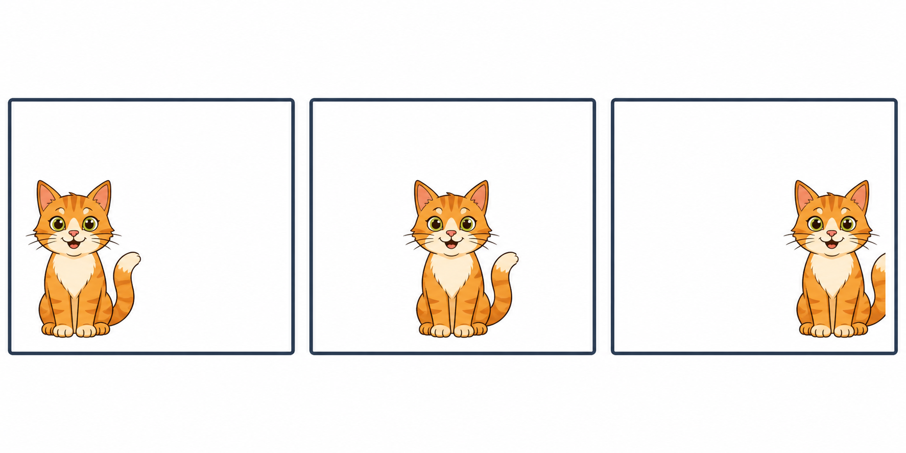
The same orange cartoon cat appears at the left, centre, and right of three otherwise identical framed images.

Equivariance

Let \(T_\Delta\) translate an input by \(\Delta\) positions.

\[ F(T_\Delta X)=T_\Delta F(X) \]

A convolutional feature map moves with the input pattern.

How can y keep the length of x?

def conv1d(x, w, padding=(0, 0)):

    P_left, P_right = padding
    x_pad = np.pad(x, (P_left, P_right), mode="constant")
    K = w.size
    L_out = x_pad.size - K + 1
    y = np.zeros(L_out)

    for i in range(L_out):
        for j in range(K):
            y[i] += x_pad[i + j] * w[j]

    return y

up_map_same = conv1d(x_walking, kernel_up, padding=(2, 2))

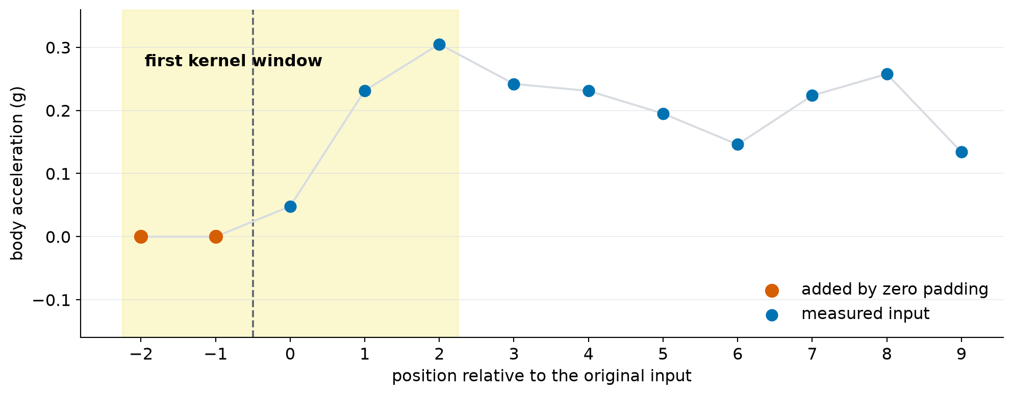
\[ L_{\mathrm{out}}=L+P_{\mathrm{left}}+P_{\mathrm{right}}-K+1 \]

Values that were not measured

Show plotting code
P = 2
shown = 10
padded_index = np.arange(-P, shown)
padded_values = np.concatenate([np.zeros(P), x_walking[:shown]])

fig, ax = plt.subplots(figsize=(10.5, 4.2))
ax.axvspan(-P - 0.25, 2.25, color=HIGHLIGHT, alpha=0.25)
ax.axvline(-0.5, color=GRAY, linestyle="--", linewidth=1.4)
ax.plot(padded_index, padded_values, color=LIGHT_GRAY, linewidth=1.5)
ax.scatter(
    padded_index[:P],
    padded_values[:P],
    color=ORANGE,
    s=85,
    label="added by zero padding",
    zorder=3,
)
ax.scatter(
    padded_index[P:],
    padded_values[P:],
    color=BLUE,
    s=65,
    label="measured input",
    zorder=3,
)
ax.text(-1.95, 0.27, "first kernel window", fontweight="bold")
ax.set_xticks(padded_index)
ax.set_xlabel("position relative to the original input")
ax.set_ylabel("body acceleration (g)")
ax.set_ylim(-0.16, 0.36)
ax.grid(axis="y", color=LIGHT_GRAY, linewidth=0.7, alpha=0.55)
ax.legend(loc="lower right")
fig.tight_layout()
plt.show()

The first ten acceleration values preceded by two artificial zeros; the first five-value kernel window includes both padded and measured values.

What happens if i advances by 2?

def conv1d(x, w, padding=(0, 0), stride=1):

    P_left, P_right = padding
    x_pad = np.pad(x, (P_left, P_right), mode="constant")
    K = w.size
    starts = range(0, x_pad.size - K + 1, stride)
    y = np.zeros(len(starts))

    for t, i in enumerate(starts):
        for j in range(K):
            y[t] += x_pad[i + j] * w[j]

    return y

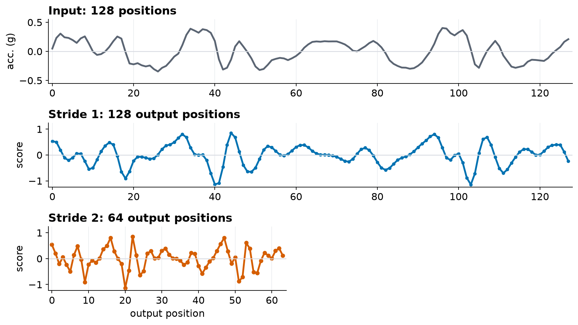
\[ L_{\mathrm{out}}= \left\lfloor\frac{L+P_{\mathrm{left}}+P_{\mathrm{right}}-K}{S}\right\rfloor+1 \]

What happens when the stride is 2?

Show plotting code
stride1_map = conv1d(x_walking, kernel_up, padding=(2, 2), stride=1)
stride2_map = conv1d(x_walking, kernel_up, padding=(2, 2), stride=2)

input_position = np.arange(x_walking.size)
stride1_position = np.arange(stride1_map.size)
stride2_position = np.arange(stride2_map.size)
score_limit = 1.08 * max(np.abs(stride1_map).max(), np.abs(stride2_map).max())

fig = plt.figure(figsize=(11.5, 6.0))
grid = fig.add_gridspec(3, 2, width_ratios=[1, 1], hspace=0.62)
input_ax = fig.add_subplot(grid[0, :])
stride1_ax = fig.add_subplot(grid[1, :])
stride2_ax = fig.add_subplot(grid[2, 0])
empty_ax = fig.add_subplot(grid[2, 1])
empty_ax.axis("off")

input_ax.plot(input_position, x_walking, color=GRAY)
input_ax.set_title("Input: 128 positions", loc="left")
input_ax.set_ylabel("acc. (g)")
input_ax.set_ylim(-0.55, 0.55)
input_ax.set_xlim(-1, 128)

stride1_ax.plot(stride1_position, stride1_map, color=BLUE)
stride1_ax.scatter(stride1_position, stride1_map, color=BLUE, s=10)
stride1_ax.set_title("Stride 1: 128 output positions", loc="left")
stride1_ax.set_ylabel("score")
stride1_ax.set_ylim(-score_limit, score_limit)
stride1_ax.set_xlim(-1, 128)

stride2_ax.plot(stride2_position, stride2_map, color=ORANGE)
stride2_ax.scatter(stride2_position, stride2_map, color=ORANGE, s=18)
stride2_ax.set_title("Stride 2: 64 output positions", loc="left")
stride2_ax.set_ylabel("score")
stride2_ax.set_xlabel("output position")
stride2_ax.set_ylim(-score_limit, score_limit)
stride2_ax.set_xlim(-1, 64)

for ax in [input_ax, stride1_ax, stride2_ax]:
    ax.axhline(0, color=LIGHT_GRAY, linewidth=1)
    ax.grid(axis="x", color=LIGHT_GRAY, linewidth=0.7, alpha=0.55)

fig.tight_layout()
plt.show()

A 128-position input and 128-position stride-one output span the full width; the 64-position stride-two output occupies only the left half.

Multiple kernels and channels

Multiple local patterns

Upward contrast

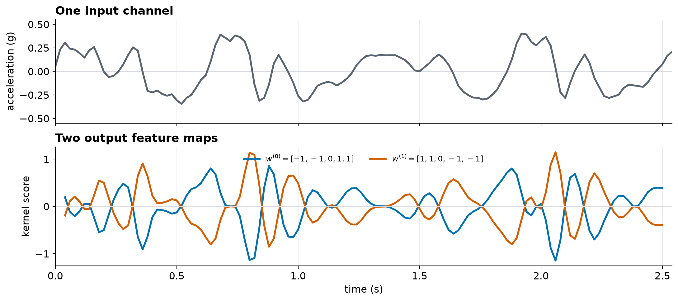
\[ w^{(0)} = [-1,-1,0,1,1] \]

The first pair is subtracted from the last pair.

Downward contrast

\[ w^{(1)} = [1,1,0,-1,-1] \]

The last pair is subtracted from the first pair.

\[ W = \begin{bmatrix}\vert & \vert\\ w^{(0)} & w^{(1)}\\ \vert & \vert\end{bmatrix} \in \mathbb{R}^{K\times C_{\mathrm{out}}} \]

How many kernels should a layer use?

  • Domain expertise can suggest a small, interpretable set.
  • More commonly, \(C_{\mathrm{out}}\) is a hyperparameter selected using validation data.
  • More kernels increase representational capacity, parameter count, memory, and computation.

The loop gains one kernel index

def conv1d(x, W, b, padding=(0, 0), stride=1):

    P_left, P_right = padding
    x_pad = np.pad(x, (P_left, P_right), mode="constant")
    K, C_out = W.shape
    starts = range(0, x_pad.size - K + 1, stride)
    Y = np.zeros((len(starts), C_out))

    for t, i in enumerate(starts):
        for m in range(C_out):
            Y[t, m] = b[m]
            for j in range(K):
                Y[t, m] += x_pad[i + j] * W[j, m]

    return Y

Each kernel creates one feature map

Show plotting code
kernels = np.column_stack([kernel_up, kernel_down])
bias = np.zeros(2)
feature_maps = conv1d(x_walking, kernels, bias)
feature_time = (np.arange(feature_maps.shape[0]) + (K - 1) / 2) / SAMPLE_RATE

fig, axes = plt.subplots(
    2,
    1,
    figsize=(11.5, 5.2),
    sharex=True,
    gridspec_kw={"height_ratios": [1, 1.15]},
)

axes[0].plot(time, x_walking, color=GRAY)
axes[0].set_title("One input channel", loc="left")
style_time_axis(
    axes[0],
    ylabel="acceleration (g)",
    ylim=(-0.55, 0.55),
)

axes[1].plot(
    feature_time,
    feature_maps[:, 0],
    color=BLUE,
    label=r"$w^{(0)}=[-1,-1,0,1,1]$",
)
axes[1].plot(
    feature_time,
    feature_maps[:, 1],
    color=ORANGE,
    label=r"$w^{(1)}=[1,1,0,-1,-1]$",
)
axes[1].axhline(0, color=LIGHT_GRAY, linewidth=1)
axes[1].grid(axis="x", color=LIGHT_GRAY, linewidth=0.7, alpha=0.55)
axes[1].set_xlim(time[0], time[-1])
axes[1].set_title("Two output feature maps", loc="left")
axes[1].set_ylabel("kernel score")
axes[1].set_xlabel("time (s)")
axes[1].legend(loc="upper center", ncol=2, fontsize=9.5)

fig.tight_layout(h_pad=0.7)
plt.show()

One body-acceleration signal above two feature maps produced by explicit upward- and downward-transition kernels.

Shapes keep everything interpretable

Object Meaning Shape
\(X\) input sequence \((L,C_{\mathrm{in}})\)
\(W\) kernel weights \((K,C_{\mathrm{in}},C_{\mathrm{out}})\)
\(b\) one bias per output channel \((C_{\mathrm{out}})\)
\(Y\) output feature maps \((L_{\mathrm{out}},C_{\mathrm{out}})\)

\[ Y[t,m] = b[m] + \sum_{j=0}^{K-1}\sum_{c=0}^{C_{\mathrm{in}}-1} \widetilde X[tS+j,c]W[j,c,m] \]

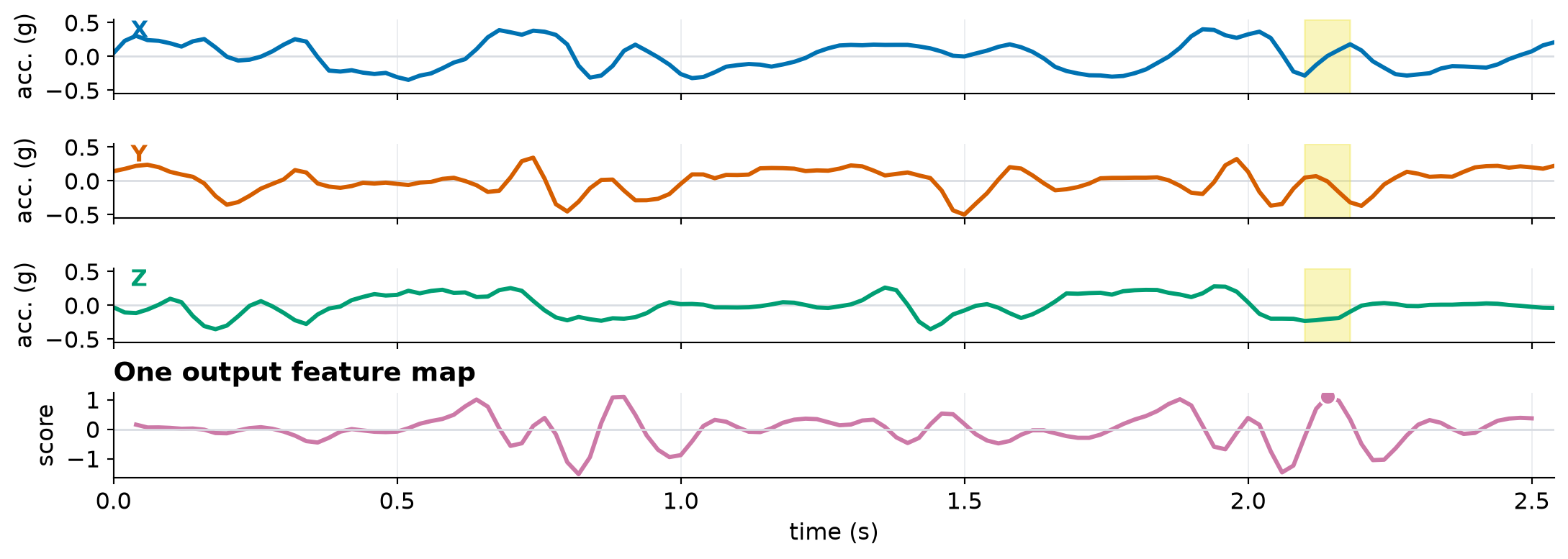
A patch spans all input channels

def conv1d(X, W, b, padding=(0, 0), stride=1):

    P_left, P_right = padding
    X_pad = np.pad(X, ((P_left, P_right), (0, 0)), mode="constant")
    K, C_in, C_out = W.shape
    starts = range(0, X_pad.shape[0] - K + 1, stride)
    Y = np.zeros((len(starts), C_out))

    for t, i in enumerate(starts):
        for m in range(C_out):
            Y[t, m] = b[m]
            for j in range(K):
                for c in range(C_in):
                    Y[t, m] += X_pad[i + j, c] * W[j, c, m]

    return Y

A kernel spans every input channel

Show example tensors and plotting code
X = walking.loc[:, ["x", "y", "z"]].to_numpy()

# One illustrative kernel: five positions, three channels, one output map.
W = np.stack(
    [kernel_up, -0.6 * kernel_up, 0.4 * kernel_up],
    axis=1,
)[:, :, np.newaxis]
b = np.zeros(1)
Y = conv1d(X, W, b, padding=(0, 0), stride=1)

multi_map = Y[:, 0]
multi_feature_time = (
    np.arange(multi_map.size) + (K - 1) / 2
) / SAMPLE_RATE
best_multi = int(np.argmax(multi_map))
start = best_multi
stop = start + K

fig, axes = plt.subplots(
    4,
    1,
    figsize=(11.5, 4.2),
    sharex=True,
    gridspec_kw={"height_ratios": [1, 1, 1, 1.15]},
)

for ax, channel, color in zip(
    axes[:3], ["x", "y", "z"], [BLUE, ORANGE, GREEN]
):
    ax.plot(time, walking[channel], color=color)
    ax.axvspan(
        time[start],
        time[stop - 1],
        color=HIGHLIGHT,
        alpha=0.35,
    )
    ax.text(
        0.012,
        0.76,
        channel.upper(),
        transform=ax.transAxes,
        color=color,
        fontweight="bold",
    )
    style_time_axis(ax, ylabel="acc. (g)", ylim=(-0.55, 0.55))

axes[3].plot(multi_feature_time, multi_map, color=PURPLE)
axes[3].scatter(
    multi_feature_time[best_multi],
    multi_map[best_multi],
    color=PURPLE,
    edgecolor="white",
    linewidth=1.2,
    s=70,
    zorder=3,
)
axes[3].axhline(0, color=LIGHT_GRAY, linewidth=1)
axes[3].grid(axis="x", color=LIGHT_GRAY, linewidth=0.7, alpha=0.55)
axes[3].set_xlim(time[0], time[-1])
axes[3].set_ylabel("score")
axes[3].set_xlabel("time (s)")
axes[3].set_title("One output feature map", loc="left")

fig.tight_layout(h_pad=0.35)
plt.show()

Three synchronized body-acceleration channels with one shared temporal window and the resulting feature map.

Stacking and pooling

What do X and Y represent?

\[ X \;\xrightarrow{\;\text{convolution}+b\;}\; Z \;\xrightarrow{\;g\;}\; Y \]

\[ X^{(\ell+1)}=Y^{(\ell)} \]

  • \(X\): input to one layer;
  • \(Z\): pre-activation scores;
  • \(Y=g(Z)\): output activations; and
  • the channels of \(Y^{(\ell)}\) become the channels of the next layer’s input.

How to combine feature maps?

def relu(Z):
    return np.maximum(Z, 0)

X0 = x_walking[:, np.newaxis]
W1 = kernels[:, np.newaxis, :]
b1 = np.zeros(2)
Z1 = conv1d(X0, W1, b1)
Y1 = relu(Z1)

W2 = np.zeros((K, 2, 1))

W2[:2, 0, 0] = 0.5     # earlier upward evidence
W2[-2:, 1, 0] = 0.5    # later downward evidence

b2 = np.array([-0.8])
Z2 = conv1d(Y1, W2, b2)
Y2 = relu(Z2)

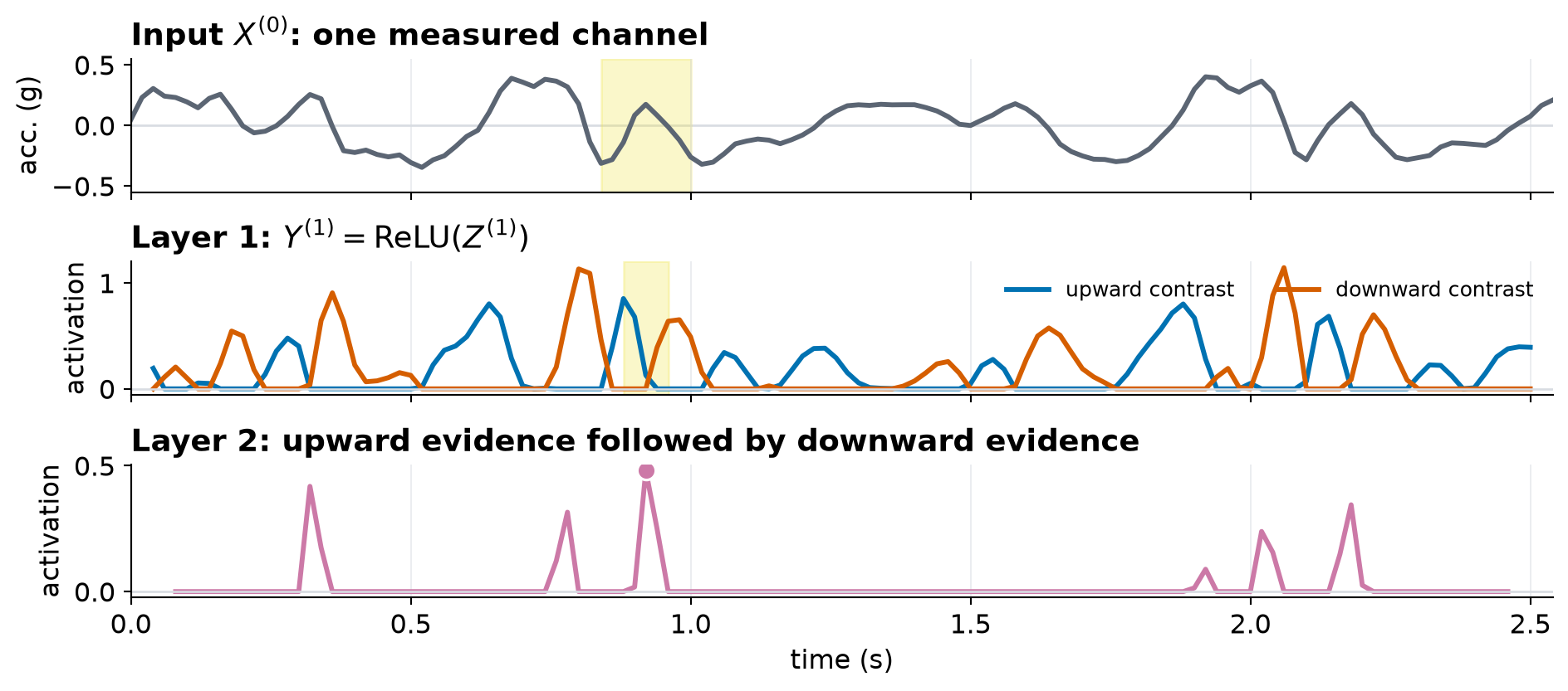
Layers detect patterns of patterns

Show code
time1 = (np.arange(Y1.shape[0]) + (K - 1) / 2) / SAMPLE_RATE
time2 = (np.arange(Y2.shape[0]) + (K - 1)) / SAMPLE_RATE
best_pattern = int(np.argmax(Y2[:, 0]))
receptive_start = best_pattern
receptive_stop = best_pattern + 2 * K - 1

fig, axes = plt.subplots(3, 1, figsize=(10.0, 4.5), sharex=True)

axes[0].plot(time, X0[:, 0], color=GRAY)
axes[0].axvspan(
    time[receptive_start],
    time[receptive_stop - 1],
    color=HIGHLIGHT,
    alpha=0.28,
)
axes[0].set_title(r"Input $X^{(0)}$: one measured channel", loc="left")
style_time_axis(axes[0], ylabel="acc. (g)", ylim=(-0.55, 0.55))

axes[1].plot(time1, Y1[:, 0], color=BLUE, label="upward contrast")
axes[1].plot(time1, Y1[:, 1], color=ORANGE, label="downward contrast")
axes[1].axvspan(
    time1[best_pattern],
    time1[best_pattern + K - 1],
    color=HIGHLIGHT,
    alpha=0.28,
)
axes[1].set_title(
    r"Layer 1: $Y^{(1)}=\operatorname{ReLU}(Z^{(1)})$",
    loc="left",
)
axes[1].set_ylabel("activation")
axes[1].axhline(0, color=LIGHT_GRAY, linewidth=1)
axes[1].grid(axis="x", color=LIGHT_GRAY, linewidth=0.7, alpha=0.55)
axes[1].legend(loc="upper right", ncol=2, fontsize=9.5)

axes[2].plot(time2, Y2[:, 0], color=PURPLE)
axes[2].scatter(
    time2[best_pattern],
    Y2[best_pattern, 0],
    color=PURPLE,
    edgecolor="white",
    linewidth=1.2,
    s=70,
    zorder=3,
)
axes[2].set_title(
    "Layer 2: upward evidence followed by downward evidence",
    loc="left",
)
axes[2].set_ylabel("activation")
axes[2].set_xlabel("time (s)")
axes[2].axhline(0, color=LIGHT_GRAY, linewidth=1)
axes[2].grid(axis="x", color=LIGHT_GRAY, linewidth=0.7, alpha=0.55)
axes[2].set_xlim(time[0], time[-1])

fig.tight_layout(h_pad=0.65)
plt.show()

One acceleration input produces upward and downward ReLU activations in layer one; layer two combines earlier upward and later downward evidence into one activation map.

What does the bias change?

\[ Y[i,m] = \sum_{j=0}^{K-1}x[i+j] W[j,m] + b[m] \]

Patch or receptive field?

  • A patch or window is the slice of a layer’s current input used at one kernel placement.
  • A unit’s receptive field is the set of original-input positions that can influence it.

For unit stride and no dilation,

\[ R_1=K_1,\qquad R_2=R_1+(K_2-1). \]

With two kernels of length 5, one second-layer activation can depend on \(5+(5-1)=9\) original positions.

Summarizing the neighbourhood

def max_pool1d(y, pool_size=2, stride=2):

    L_out = (len(y) - pool_size) // stride + 1
    p = np.zeros(L_out)

    for t in range(L_out):
        i = t * stride
        window = y[i : i + pool_size]
        p[t] = max(window)

    return p

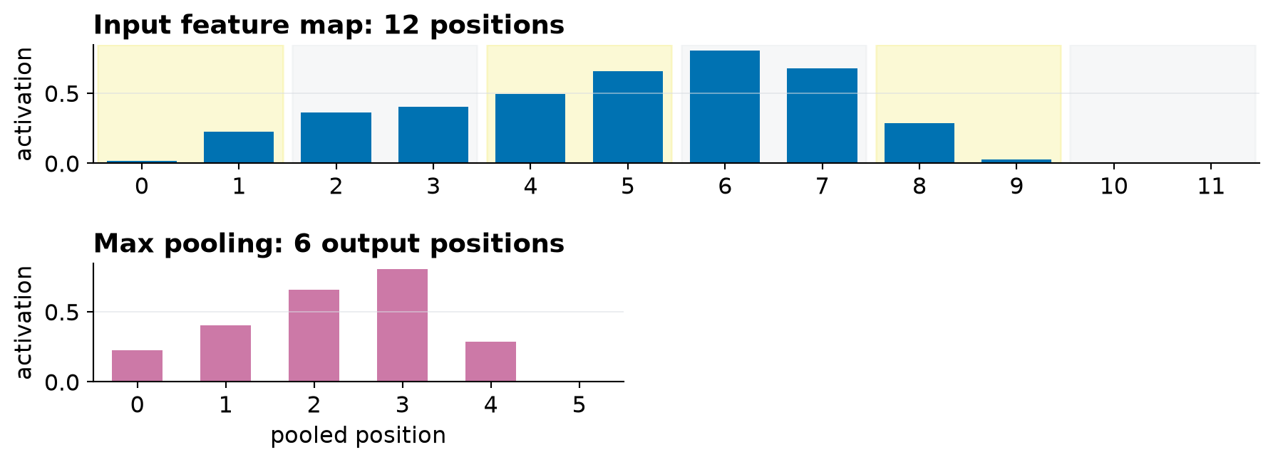
\[ p[t]=\max_{0\leq j<P} y[tS+j] \]

Pooling reduces sequence length

Show plotting code
# Select a short region containing varied positive activations.
pool_start = 24
pool_input = np.maximum(up_map[pool_start : pool_start + 12], 0)
pool_output = max_pool1d(pool_input, pool_size=2, stride=2)

fig = plt.figure(figsize=(11.0, 3.2))
grid = fig.add_gridspec(2, 2, width_ratios=[1, 1], hspace=0.85)
input_ax = fig.add_subplot(grid[0, :])
pooled_ax = fig.add_subplot(grid[1, 0])
empty_ax = fig.add_subplot(grid[1, 1])
empty_ax.axis("off")

for pair in range(6):
    color = HIGHLIGHT if pair % 2 == 0 else LIGHT_GRAY
    input_ax.axvspan(
        2 * pair - 0.45,
        2 * pair + 1.45,
        color=color,
        alpha=0.22,
    )

input_ax.bar(np.arange(12), pool_input, color=BLUE, width=0.72)
input_ax.set_title("Input feature map: 12 positions", loc="left")
input_ax.set_ylabel("activation")
input_ax.set_xticks(np.arange(12))
input_ax.set_xlim(-0.5, 11.5)
input_ax.grid(axis="y", color=LIGHT_GRAY, linewidth=0.7, alpha=0.55)

pooled_ax.bar(np.arange(6), pool_output, color=PURPLE, width=0.58)
pooled_ax.set_title("Max pooling: 6 output positions", loc="left")
pooled_ax.set_ylabel("activation")
pooled_ax.set_xlabel("pooled position")
pooled_ax.set_xticks(np.arange(6))
pooled_ax.set_xlim(-0.5, 5.5)
pooled_ax.grid(axis="y", color=LIGHT_GRAY, linewidth=0.7, alpha=0.55)

fig.tight_layout()
plt.show()

Twelve nonnegative activations span the full width; six max-pooled outputs occupy half the width below them.

Impact on length

Operation Parameters Channels
Stride weighted sum kernel weights and bias may change
Pooling fixed maximum or mean none usually unchanged

From features to predictions

How do feature maps predict?

\[ Y\in\mathbb{R}^{L_{\mathrm{out}}\times C_{\mathrm{out}}} \;\xrightarrow{\;\text{global pooling}\;}\; h\in\mathbb{R}^{C_{\mathrm{out}}} \;\xrightarrow{\;\text{Dense}\;}\; z\in\mathbb{R} \;\xrightarrow{\;\sigma\;}\; \widehat p_{\mathrm{walking}} \]

\[ h[m]=\max_i Y[i,m], \qquad z=\sum_m v[m]h[m]+a, \qquad \widehat p_{\mathrm{walking}}=\sigma(z). \]

Do we need to know where a feature occurred, or only whether it occurred?

What changes under translation?

Let \(T_\Delta\) translate an input by \(\Delta\) positions.

Equivariance

\[ F(T_\Delta X)=T_\Delta F(X) \]

A convolutional feature map moves with the input pattern.

Invariance

\[ G(T_\Delta Y)=G(Y) \]

A position-aggregating readout can preserve the final decision.

Prediction requires a head

def sigmoid(z):
    return 1 / (1 + np.exp(-z))

def predict_walking(Y, v, a):
    C_out = Y.shape[1]
    h = np.zeros(C_out)
    for m in range(C_out):
        h[m] = max(Y[:, m])  # one value per feature map

    z = h @ v + a            # Dense layer
    return sigmoid(z)

\[ \text{signal} \rightarrow \text{convolutional layers} \rightarrow \text{global pooling} \rightarrow \text{Dense} \rightarrow \text{prediction} \]

How are all parameters learned?

\[ \text{labelled examples} \rightarrow \text{forward pass} \rightarrow \text{loss} \]

\[ \text{loss} \rightarrow \text{backpropagation} \rightarrow \text{parameter update} \rightarrow \text{repeat} \]

  • Learned: every kernel weight, every output-channel bias, and the prediction-head weights and bias.
  • Specified: padding, stride, pooling rule, activation function, and layer sizes.

More dimensions add indices

\[ \begin{aligned} \text{1D: } & W[j,c,m] \\ \text{2D: } & W[j_1,j_2,c,m] \\ \text{3D: } & W[j_1,j_2,j_3,c,m] \end{aligned} \]

Each kernel still:

  1. selects a local patch;
  2. multiplies matching values and weights;
  3. sums over local positions and input channels; and
  4. produces one value in one output feature map.

Can a phone recognize walking?

\[ X \rightarrow \text{local features} \rightarrow \text{feature hierarchy} \rightarrow \text{global summary} \rightarrow \widehat p_{\mathrm{walking}} \]

Yes—after the kernels, biases, and prediction head have been learned from labelled examples.

Prologue

Summary

  • Locality and sharing: the same kernel examines every local patch, producing a feature map with relatively few parameters.
  • Channels: each kernel spans all input channels and produces one output feature map.
  • Geometry: padding controls boundaries; stride and pooling control resolution and retained positional detail.

Summary (continued)

  • Hierarchy: stacked layers compose simpler features and enlarge receptive fields.
  • Prediction: convolution is translation equivariant; position aggregation can support invariant predictions, and a prediction head produces the final output.
  • Learning: backpropagation learns every kernel, weight, and bias jointly.

Further Reading

  • Understanding Deep Learning (Prince 2023) is a recently published textbook focused on the foundational concepts of deep learning.

  • It begins with fundamental principles and extends to contemporary topics such as transformers, diffusion models, graph neural networks, autoencoders, adversarial networks, and reinforcement learning.

  • The textbook aims to help readers comprehend these concepts without delving excessively into theoretical details.

  • It includes sixty-eight Python notebook exercises.

  • The book follows a “read-first, pay-later” model.

Resources

StatQuest

Next lecture

  • We will introduce search.

References

Géron, Aurélien. 2019. Hands-on Machine Learning with Scikit-Learn, Keras, and TensorFlow. 2nd ed. O’Reilly Media.
Krizhevsky, Alex, Ilya Sutskever, and Geoffrey E Hinton. 2012. “ImageNet Classification with Deep Convolutional Neural Networks.” In Advances in Neural Information Processing Systems, edited by F. Pereira, C. J. Burges, L. Bottou, and K. Q. Weinberger, vol. 25. Curran Associates, Inc. https://proceedings.neurips.cc/paper_files/paper/2012/file/c399862d3b9d6b76c8436e924a68c45b-Paper.pdf.
Prince, Simon J. D. 2023. Understanding Deep Learning. The MIT Press. http://udlbook.com.
Russell, Stuart, and Peter Norvig. 2020. Artificial Intelligence: A Modern Approach. 4th ed. Pearson. http://aima.cs.berkeley.edu/.
Simonyan, Karen, and Andrew Zisserman. 2015. “Very Deep Convolutional Networks for Large-Scale Image Recognition.” International Conference on Learning Representations.

Appendix: Well-known convolutional neural networks

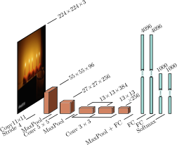
AlexNet

Krizhevsky et al. (2012)

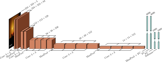
VGG

Simonyan and Zisserman (2015)

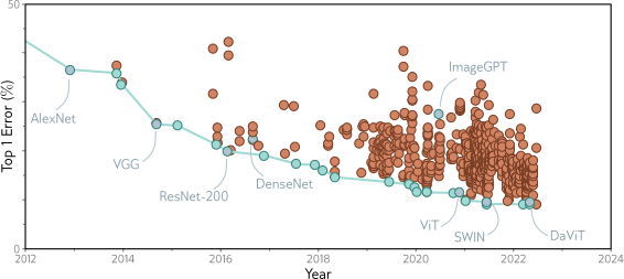
ConvNets Performance

Marcel Turcotte

Marcel.Turcotte@uOttawa.ca

School of Electrical Engineering and Computer Science (EECS)

University of Ottawa