Training neural networks: challenges and practical choices

CSI 4106 - Fall 2026

Marcel Turcotte

Version: Oct 31, 2026 13:34

Preamble

Message of the Day

Learning objectives

  • Explain how loss landscapes, activation derivatives, and initialization affect optimization.
  • Distinguish vanishing gradients, exploding gradients, and overfitting.
  • Choose output activations and losses for regression, binary, multilabel, and multiclass tasks.
  • Explain L1, L2, dropout, and early stopping, and interpret their effects in code.
  • Compare SimplerMLP with SimpleMLP and distinguish inference from further learning.
  • Recognize catastrophic forgetting and explain how replay can improve retention.

Loss landscapes and optimization

We have gradients. What could still go wrong?

Backpropagation was popularized in 1986. Why did deep learning take off much later?

  • The loss landscape describes the objective as a function of the parameters.
  • A gradient describes the local change in that objective.
  • Progress also depends on the starting parameters and the learning rate.

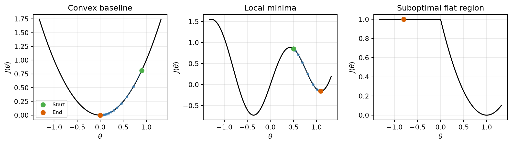
Where will gradient descent take us?

Start at each green point. With a small fixed learning rate, where might the updates stop?

Show code
import numpy as np
import matplotlib.pyplot as plt

def gradient_descent_1d(gradient, start, learning_rate, steps, clip_value=None):
    trajectory = [float(start)]
    for _ in range(steps):
        g = float(gradient(trajectory[-1]))
        if not np.isfinite(g):
            break  # The toy objective has no finite derivative here.
        if clip_value is not None:
            g = np.clip(g, -clip_value, clip_value)
        trajectory.append(trajectory[-1] - learning_rate * g)
    return np.asarray(trajectory)

def plot_landscape(objective, trajectory, ax, title, show_trajectory=True):
    left = min(-1.2, trajectory.min())
    right = max(1.2, trajectory.max())
    padding = 0.05 * (right - left)
    theta = np.linspace(left - padding, right + padding, 800)
    ax.plot(theta, objective(theta), color='black', linewidth=1.5)
    if show_trajectory:
        ax.plot(trajectory, objective(trajectory), 'o-', color='#377eb8',
                markersize=3, linewidth=0.8, alpha=0.65)
    ax.scatter(trajectory[0], objective(trajectory[0]), color='#4daf4a',
               s=45, zorder=4, label='Start')
    if show_trajectory:
        ax.scatter(trajectory[-1], objective(trajectory[-1]), color='#d95f02',
                   s=45, zorder=5, label='End')
    ax.set(title=title, xlabel=r'$\theta$', ylabel=r'$J(\theta)$')
    ax.grid(alpha=0.25)
    return theta


fig, axes = plt.subplots(1, 3, figsize=(11, 3.2))
overview = [
    ('Convex baseline', lambda t: t**2, lambda t: 2*t, 0.9, 0.1),
    ('Local minima', lambda t: 0.8*np.sin(4*t)+0.5*t**2,
     lambda t: 3.2*np.cos(4*t)+t, 0.5, 0.05),
    ('Suboptimal flat region', lambda t: (np.maximum(0, t)-1)**2,
     lambda t: 2*(t-1) if t > 0 else 0.0, -0.8, 0.1)
]
for index, (ax, (_, objective, gradient, start, rate)) in enumerate(zip(axes, overview)):
    trajectory = gradient_descent_1d(gradient, start, rate, steps=60)
    plot_landscape(objective, trajectory, ax, f'Landscape {index+1}',
                   show_trajectory=False)
axes[0].legend(fontsize=8)
fig.tight_layout()
plt.show()

Three landscapes, three trajectories

Show code
fig, axes = plt.subplots(1, 3, figsize=(11, 3.2))
for ax, (title, objective, gradient, start, rate) in zip(axes, overview):
    trajectory = gradient_descent_1d(gradient, start, rate, steps=60)
    plot_landscape(objective, trajectory, ax, title)
axes[0].legend(fontsize=8)
fig.tight_layout()
plt.show()

Gradient propagation and initialization

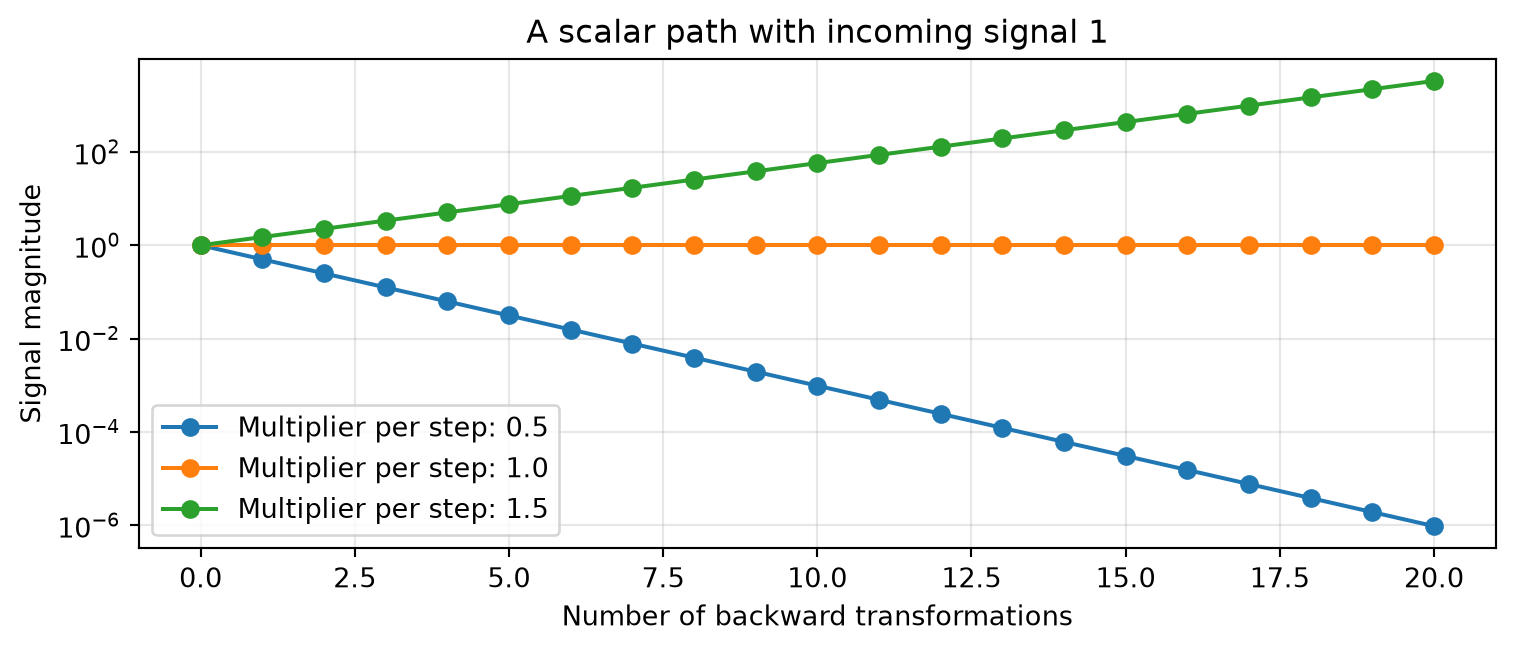
What happens along a longer path?

Lecture 13 used one hidden unit. What happens when many backward transformations are composed?

Show code
distance = np.arange(21)
fig, ax = plt.subplots(figsize=(8, 3.5))
for factor in (0.5, 1.0, 1.5):
    ax.semilogy(distance, factor**distance, 'o-', label=f'Multiplier per step: {factor}')
ax.set(xlabel='Number of backward transformations', ylabel='Signal magnitude',
       title='A scalar path with incoming signal 1')
ax.grid(alpha=0.3)
ax.legend()
fig.tight_layout()
plt.show()

Vanishing gradients

  • Backpropagation repeatedly multiplies weights and local activation derivatives.
  • Small factors can make early-layer gradients too small for effective learning.
  • Saturated sigmoid units have derivatives close to zero.

Exploding gradients

  • Repeated transformations can amplify backward signals.
  • Large gradients can cause large parameter updates and unstable training.
  • Suitable initialization and a sensible learning rate help; gradient clipping can limit updates.

Activation functions and their derivatives

Which slopes keep a backward signal useful? Does ReLU solve every problem?

Show code
# Attribution: https://github.com/ageron/handson-ml3/blob/main/10_neural_nets_with_keras.ipynb

import numpy as np
import matplotlib.pyplot as plt

from scipy.special import expit as sigmoid

def relu(z):
    return np.maximum(0, z)

def derivative(f, z, eps=0.000001):
    return (f(z + eps) - f(z - eps))/(2 * eps)

max_z = 4.5
z = np.linspace(-max_z, max_z, 200)

plt.figure(figsize=(11, 3.1))

plt.subplot(121)
plt.plot(z, relu(z), "m-.", linewidth=2, label="ReLU")
plt.plot(z, sigmoid(z), "g--", linewidth=2, label="Sigmoid")
plt.plot(z, np.tanh(z), "b-", linewidth=1, label="Tanh")
plt.grid(True)
plt.title("Activation functions")
plt.axis([-max_z, max_z, -1.65, 2.4])
plt.gca().set_yticks([-1, 0, 1, 2])
plt.legend(loc="lower right", fontsize=13)

plt.subplot(122)
plt.plot(z, derivative(sigmoid, z), "g--", linewidth=2, label="Sigmoid")
plt.plot(z, derivative(np.tanh, z), "b-", linewidth=1, label="Tanh")
plt.plot([-max_z, 0], [0, 0], "m-.", linewidth=2)
plt.plot([0, max_z], [1, 1], "m-.", linewidth=2)
plt.plot([0, 0], [0, 1], "mo", markersize=6, markerfacecolor="white")
plt.grid(True)
plt.title("Derivatives")
plt.axis([-max_z, max_z, -0.2, 1.2])

plt.show()

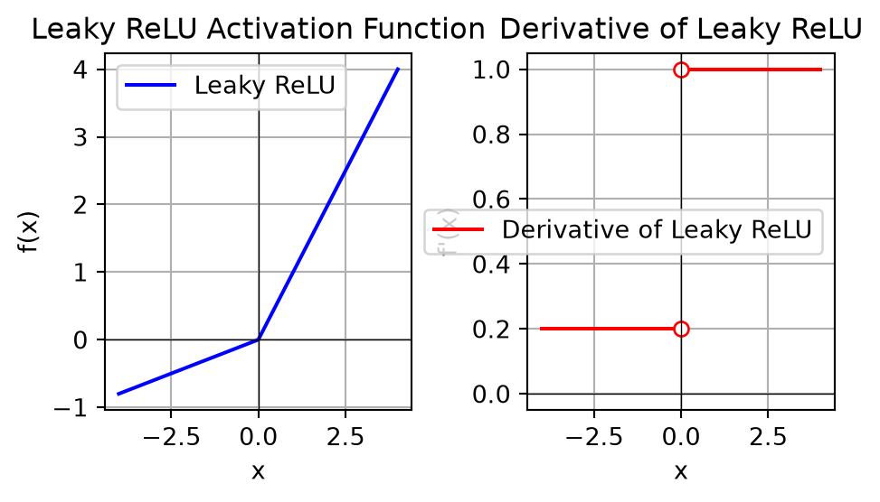
Keeping a gradient on the negative side

What if a ReLU unit stays inactive across the training examples?

Show code
import numpy as np
import matplotlib.pyplot as plt

# Define the Leaky ReLU function
def leaky_relu(x, alpha=0.2):
    return np.where(x > 0, x, alpha * x)

# Define the derivative of the Leaky ReLU function
def leaky_relu_derivative(x, alpha=0.2):
    return np.where(x > 0, 1, alpha)

# Generate a range of input values
x_values = np.linspace(-4, 4, 400)

# Compute the Leaky ReLU and its derivative
leaky_relu_values = leaky_relu(x_values)
leaky_relu_derivative_values = leaky_relu_derivative(x_values)

# Create the plot
plt.figure(figsize=(5, 3))

# Plot the Leaky ReLU
plt.subplot(1, 2, 1)
plt.plot(x_values, leaky_relu_values, label='Leaky ReLU', color='blue')
plt.title('Leaky ReLU Activation Function')
plt.xlabel('x')
plt.ylabel('f(x)')
plt.grid(True)
plt.axhline(0, color='black',linewidth=0.5)
plt.axvline(0, color='black',linewidth=0.5)
plt.legend()

# Plot the derivative of the Leaky ReLU
plt.subplot(1, 2, 2)
plt.plot([-4, 0], [0.2, 0.2], label='Derivative of Leaky ReLU', color='red')
plt.plot([0, 4], [1, 1], color='red')
plt.plot([0, 0], [0.2, 1], 'o', color='red', markerfacecolor='white')
plt.title('Derivative of Leaky ReLU')
plt.xlabel('x')
plt.ylabel("f'(x)")
plt.grid(True)
plt.axhline(0, color='black',linewidth=0.5)
plt.axvline(0, color='black',linewidth=0.5)
plt.legend()

# Show the plots
plt.tight_layout()
plt.show()

Why not start every weight at the same value?

Randomly initialized weights break symmetry between units. Biases can start at zero.

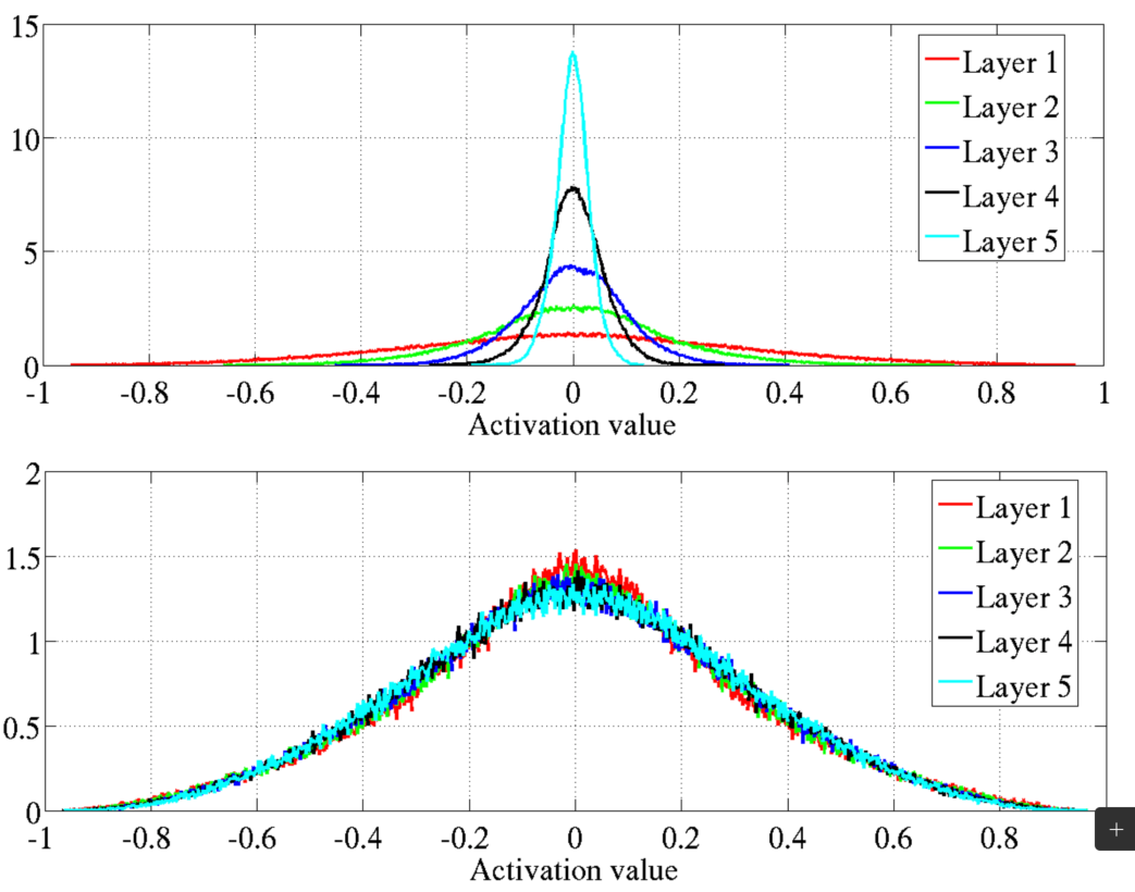
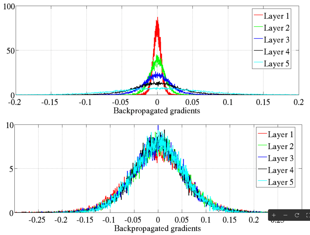
Glorot and Bengio

Random weights break symmetry. Does their scale matter?

Activations

Backward signals

He initialization

For ReLU hidden layers, He normal initialization uses

\operatorname{Var}(W)=\frac{2}{n_{\mathrm{in}}}.

def he_init(rng, fan_in, fan_out):
    std = np.sqrt(2.0 / fan_in)
    return rng.normal(0.0, std, size=(fan_in, fan_out))

Which choices help gradients propagate?

  • Alternative activation functions: Rectified Linear Unit (ReLU) and its variants (e.g., Leaky ReLU, Parametric ReLU, and Exponential Linear Unit).

  • Weight Initialization: Xavier (Glorot) or He initialization.

Gradient clipping

How could we limit an excessively large gradient-descent step while preserving its direction?

For a gradient vector g and threshold c>0:

\widetilde g = \begin{cases} g, & \|g\|_2\leq c,\\ c\,g/\|g\|_2, & \|g\|_2>c. \end{cases}

The update uses \widetilde g. Its norm is bounded by c.

optimizer = keras.optimizers.SGD(learning_rate=0.01, global_clipnorm=1.0)

Learning-rate decay

Could smaller steps help later in training? What if we reduce them too soon?

At epoch t=1,2,\ldots, with decay factor 0<\gamma<1:

\alpha_t=\alpha_1\gamma^{t-1}.

if self.lr_decay is not None:
    self.lr = self.base_lr * self.lr_decay ** (ep - 1)

Output layers

Should the output activation also change?

We replaced a hidden sigmoid with ReLU. Should we do the same at the output?

For regression, the output must match the target’s dimensions and range:

  • # of output neurons:
    • 1 per dimension
  • Output layer activation function:
    • Linear for unconstrained targets; ReLU/softplus for nonnegative targets; sigmoid/tanh for bounded targets.
  • Loss function:

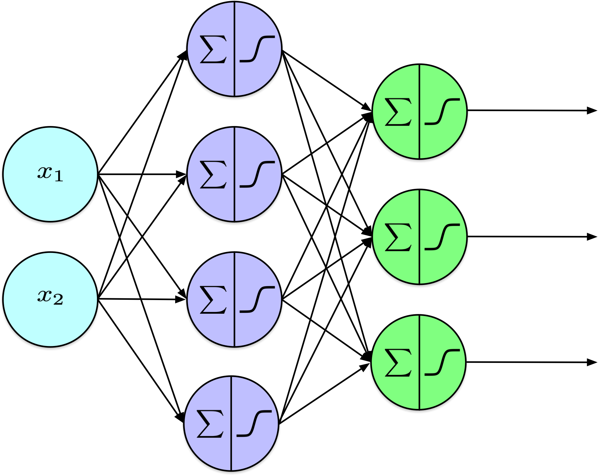
Can these probabilities describe one exclusive choice?

Separate sigmoids give [0.8,\;0.7,\;0.1]. Could several labels apply? Could exactly one class apply?

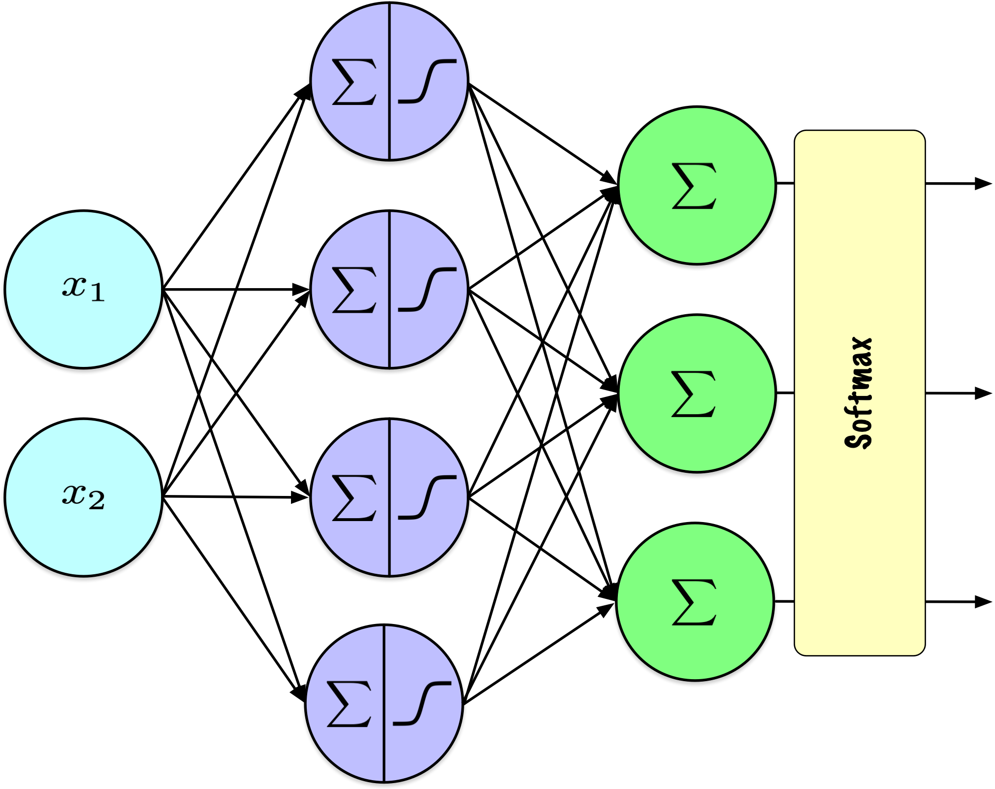
One shared output distribution

What properties should the output have when exactly one of K classes is correct?

From scores to a probability distribution

The softmax function is an activation function used in multi-class classification problems to convert a vector of raw scores into probabilities that sum to 1.

Given K output logits \mathbf{z} = [z_1, z_2, \ldots, z_K]:

\hat p_k=\operatorname{softmax}(\mathbf{z})_k = \frac{e^{z_k}}{\sum_{j=1}^{K} e^{z_j}}

Here \hat p_k is the predicted probability of class k.

What do differences between scores imply?

Which class wins? How does the gap between scores affect its probability?

z_1 z_2 z_3 \hat p_1 \hat p_2 \hat p_3 \sum
1.47 -0.39 0.22 0.69 0.11 0.20 1.00
5.00 6.00 4.00 0.24 0.67 0.09 1.00
0.90 0.80 1.10 0.32 0.29 0.39 1.00
-2.00 2.00 -3.00 0.02 0.98 0.01 1.00

Limitations

What limitations can you think of?

Our Fashion-MNIST classifier receives an image of a handwritten 7. What will it predict?

Softmax distributes all probability among the known classes. There is no built-in “none of these” output.

Can we trust the probabilities?

Among many predictions made with approximately 90% confidence, what proportion should be correct?

Approximately 90%, if the model is calibrated.

Probabilities summing to one do not guarantee calibration.

Same predicted class, same loss?

The true class is Setosa. Both predictions select it:

  • [0.25,\;\mathbf{0.51},\;0.24]
  • [0.005,\;\mathbf{0.99},\;0.005]

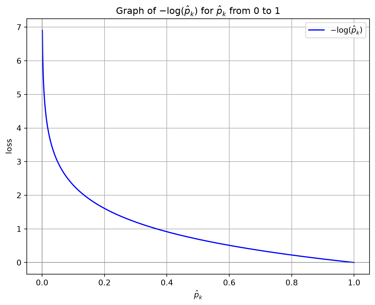
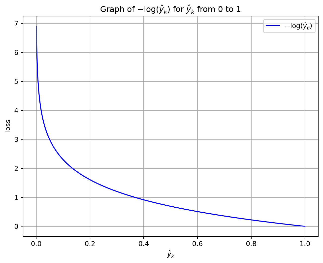
Cross-entropy rewards probability assigned to the true class:

\ell = -\sum_{k=1}^{K} y_k \log(\hat p_k)

One-hot target: y. Predicted class probabilities: \hat p_k.

Cross-entropy: a worked example

  • Classification Problem: 3 classes
    • Versicolour, Setosa, Virginica.
  • One-Hot Encoding:
    • Setosa = [0, 1, 0].
  • Softmax Outputs & Loss:
    • [0.22,\mathbf{0.7}, 0.08]: Loss = -\log(0.7) = 0.3567.
    • [0.7, \mathbf{0.22}, 0.08]: Loss = -\log(0.22) = 1.5141.
    • [0.7, \mathbf{0.08}, 0.22]: Loss = -\log(0.08) = 2.5257.

How strongly should confident mistakes be penalized?

Show code
import numpy as np
import matplotlib.pyplot as plt

# Generate an array of p values from just above 0 to 1
p_values = np.linspace(0.001, 1, 1000)

# Compute the natural logarithm of each p value
ln_p_values = - np.log(p_values)

# Plot the graph
plt.figure(figsize=(8, 6))
plt.plot(p_values, ln_p_values, label=r'$-\log(\hat p_k)$', color='b')

# Add labels and title
plt.xlabel(r'$\hat p_k$')
plt.ylabel(r'loss')
plt.title(r'Graph of $-\log(\hat p_k)$ for $\hat p_k$ from 0 to 1')
plt.grid(True)
plt.axhline(0, color='gray', lw=0.5)  # Add horizontal line at y=0
plt.axvline(0, color='gray', lw=0.5)  # Add vertical line at x=0

# Display the plot
plt.legend()
plt.show()

From one example to a dataset

For a dataset with N examples, the average cross-entropy loss over all examples is computed as:

J = -\frac{1}{N} \sum_{i=1}^{N} \sum_{k=1}^{K} y_{i,k} \log(\hat p_{i,k})

Where:

  • i indexes over the different examples in the dataset.
  • y_{i,k} and \hat p_{i,k} are the true and predicted probabilities for class k of example i, respectively.

Matching classification outputs and losses

Task Output units Activation Loss
Binary One Sigmoid Binary cross-entropy
Multi-label One per label Separate sigmoids Binary cross-entropy
Multiclass One per class Shared softmax Categorical cross-entropy

The task determines what the outputs mean and which data loss to minimize.

Further viewing: argmax and softmax

Regularization

Definition

Regularization is any modification to a learning algorithm intended to reduce its generalization error.

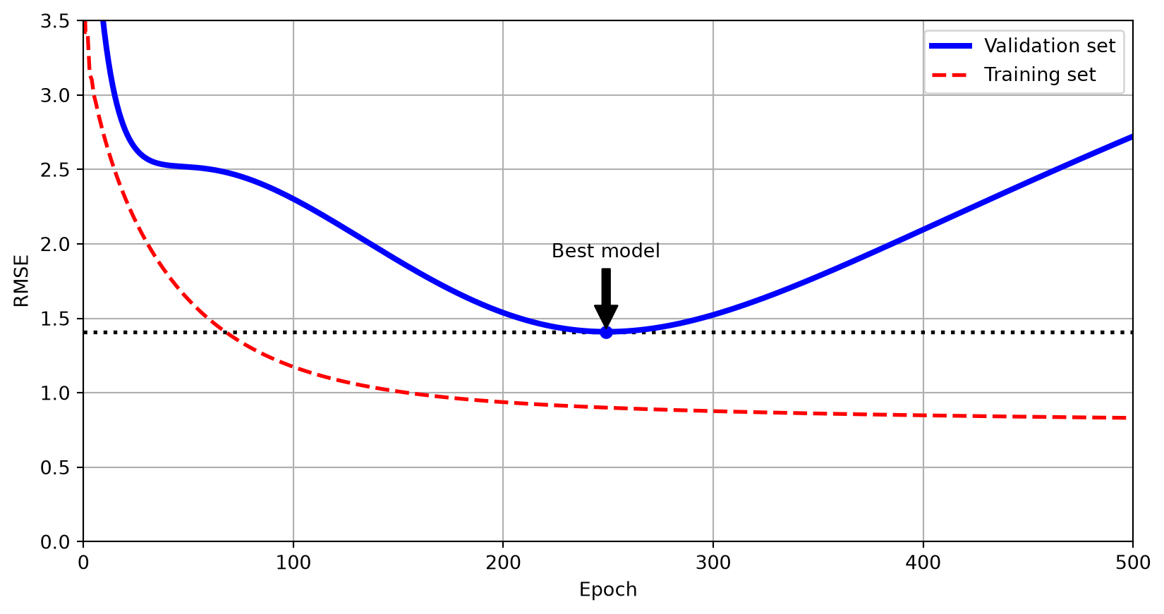
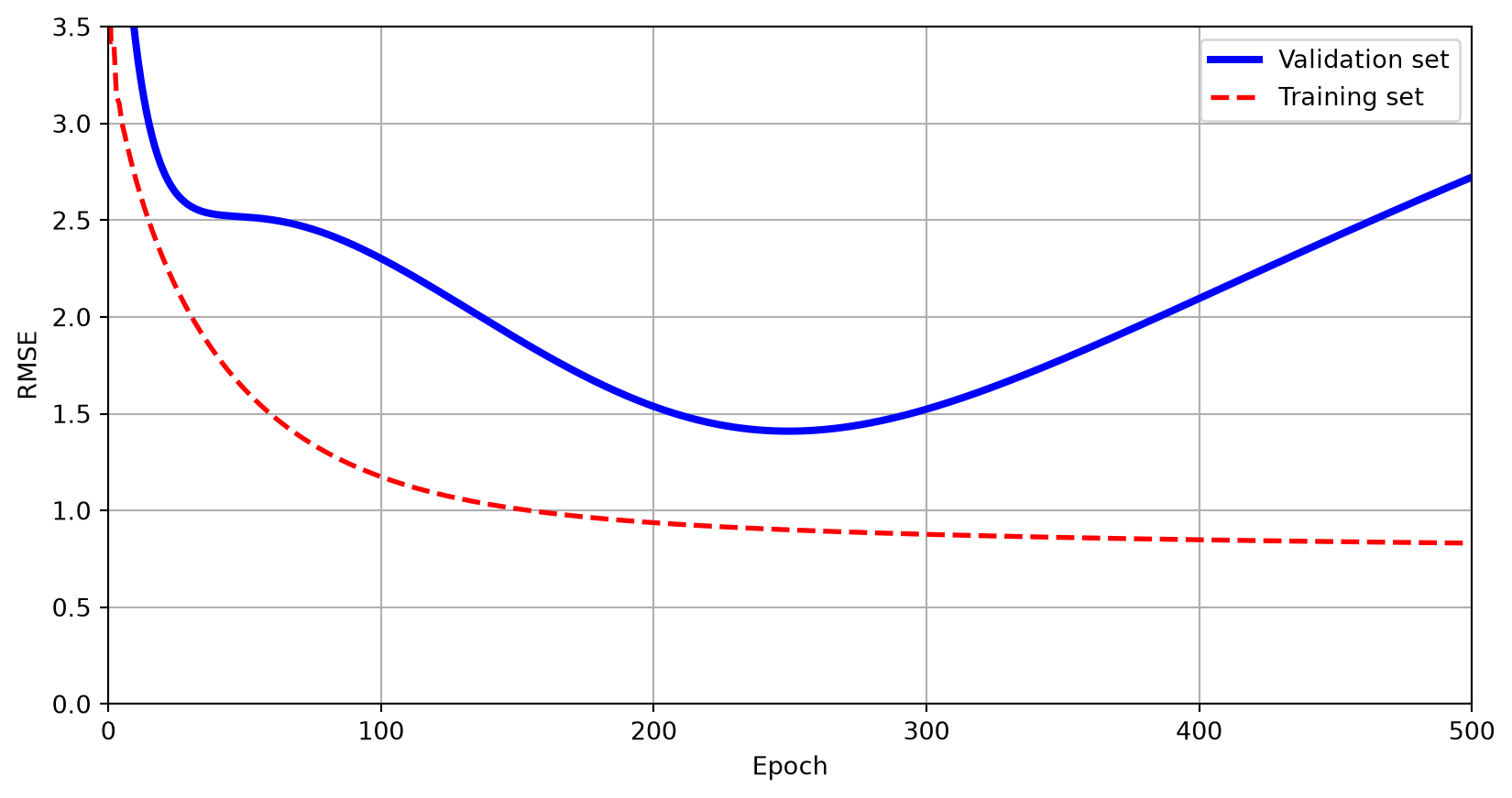
Which checkpoint would you deploy?

Training error keeps decreasing. Does the validation curve support training longer?

Show code
from copy import deepcopy
from sklearn.metrics import root_mean_squared_error
from sklearn.preprocessing import StandardScaler
from sklearn.pipeline import make_pipeline
from sklearn.preprocessing import PolynomialFeatures
from sklearn.linear_model import SGDRegressor

# Construct noisy quadratic data and reserve validation examples.
np.random.seed(42)
m = 100
X = 6 * np.random.rand(m, 1) - 3
y = 0.5 * X ** 2 + X + 2 + np.random.randn(m, 1)
X_train, y_train = X[: m // 2], y[: m // 2, 0]
X_valid, y_valid = X[m // 2 :], y[m // 2 :, 0]

preprocessing = make_pipeline(PolynomialFeatures(degree=90, include_bias=False),
                              StandardScaler())
X_train_prep = preprocessing.fit_transform(X_train)
X_valid_prep = preprocessing.transform(X_valid)
sgd_reg = SGDRegressor(penalty=None, eta0=0.002, random_state=42)
n_epochs = 500
best_valid_rmse = float('inf')
train_errors, val_errors = [], []  # extra code – it's for the figure below

for epoch in range(n_epochs):
    sgd_reg.partial_fit(X_train_prep, y_train)
    y_valid_predict = sgd_reg.predict(X_valid_prep)
    val_error = root_mean_squared_error(y_valid, y_valid_predict)
    if val_error < best_valid_rmse:
        best_valid_rmse = val_error
        best_model = deepcopy(sgd_reg)

    # extra code – we evaluate the train error and save it for the figure
    y_train_predict = sgd_reg.predict(X_train_prep)
    train_error = root_mean_squared_error(y_train, y_train_predict)
    val_errors.append(val_error)
    train_errors.append(train_error)

# extra code – this section generates and saves Figure 4–20
best_epoch = np.argmin(val_errors)
plt.plot(val_errors, "b-", linewidth=3, label="Validation set")
plt.plot(train_errors, "r--", linewidth=2, label="Training set")
plt.legend(loc="upper right")
plt.xlabel("Epoch")
plt.ylabel("RMSE")
plt.axis([0, n_epochs, 0, 3.5])
plt.grid()
plt.show()

Why regularize?

An appropriate loss and effective updates can still produce overfitting.

  • Training loss measures fit to the supplied examples.
  • Validation performance helps identify choices that generalize.
  • Stronger regularization can also cause underfitting.

Early stopping

How could the validation curve become a stopping rule?

Monitor a validation metric. Stop after a chosen number of epochs without meaningful improvement, and recover the best parameters.

Stop and restore the best parameters

For a compiled Keras model with prepared training and validation data:

early_stopping = keras.callbacks.EarlyStopping(
    monitor="val_loss", patience=5, restore_best_weights=True)
    
model.fit(X_train, y_train, validation_data=(X_valid, y_valid),
          epochs=100, callbacks=[early_stopping])

Adding a penalty to the objective

Besides choosing when to stop, can we influence which solutions training prefers?

J_{\mathrm{reg}}(W,b)=J_{\mathrm{data}}(W,b)+\Omega(W).

The data loss matches the prediction task. The penalty discourages selected weight configurations.

How could we measure weight size?

Would these two weight vectors receive the same penalty?

Weights Sum of absolute values Sum of squares
(4,0) 4 16
(2,2) 4 8

L1 uses \|\mathbf w\|_1=\sum_j|w_j|; the usual L2 penalty uses \|\mathbf w\|_2^2=\sum_j w_j^2.

\ell_1 and \ell_2 regularization

Let \mathbf w collect all weight entries. The nonnegative coefficients \lambda_1 and \lambda_2 control the penalties; zero disables the corresponding term.

J_{\mathrm{reg}}=J_{\mathrm{data}}(W,b) +\lambda_1\|\mathbf w\|_1 +\frac{\lambda_2}{2}\|\mathbf w\|_2^2.

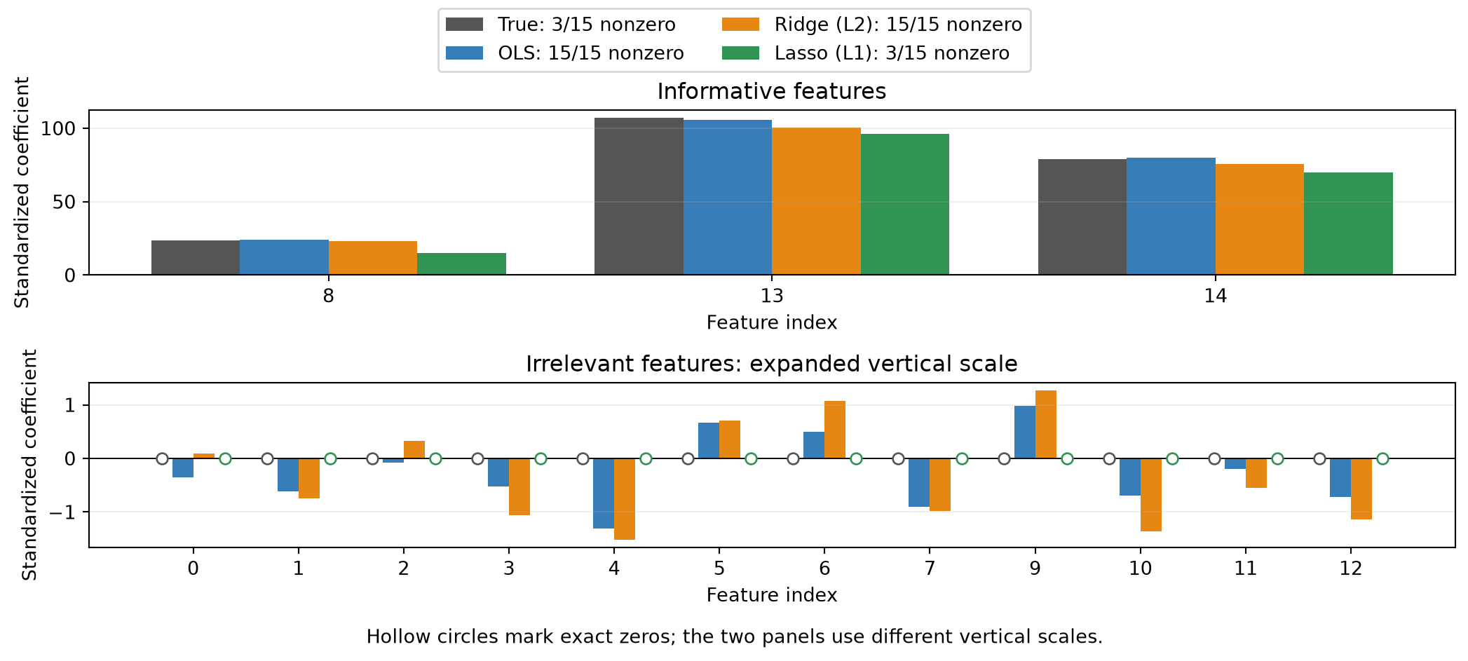
Shrinkage and sparsity

  • \ell_1 Regularization:
    • Encourages sparsity; suitable solvers can set coefficients exactly to zero.
    • Can support feature selection, particularly in linear models.
  • \ell_2 Regularization:
    • Promotes small, distributed weights for stability.
    • Shrinks weights collectively and usually retains a dense solution.

Which coefficients actually disappear?

Show code
import numpy as np
import matplotlib.pyplot as plt
from sklearn.datasets import make_regression
from sklearn.linear_model import LinearRegression, Ridge, Lasso
from sklearn.preprocessing import StandardScaler

X, y, true_coef = make_regression(n_samples=200, n_features=15, n_informative=3,
                                 noise=10.0, coef=True, random_state=42)
scaler = StandardScaler()
X_scaled = scaler.fit_transform(X)

# Express the known coefficients in the same coordinates as the fitted models.
true_coef_scaled = true_coef * scaler.scale_
coefficient_models = {
    'OLS': LinearRegression().fit(X_scaled, y),
    'Ridge (L2)': Ridge(alpha=10.0).fit(X_scaled, y),
    'Lasso (L1)': Lasso(alpha=10.0).fit(X_scaled, y)
}

series = [('True', true_coef_scaled)] + [
    (name, fitted.coef_) for name, fitted in coefficient_models.items()
]
colors = ['#555555', '#377eb8', '#e68613', '#319354']
groups = [
    (true_coef != 0, 'Informative features'),
    (true_coef == 0, 'Irrelevant features: expanded vertical scale')
]
fig, axes = plt.subplots(2, 1, figsize=(11, 4.8))
for ax, (mask, title) in zip(axes, groups):
    feature_indices = np.flatnonzero(mask)
    positions = np.arange(len(feature_indices))
    for offset, ((name, values), color) in enumerate(zip(series, colors)):
        x_positions = positions + (offset-1.5)*0.2
        nonzero = np.count_nonzero(values)
        ax.bar(x_positions, values[mask], width=0.2, color=color,
               label=f'{name}: {nonzero}/15 nonzero')
        zeros = values[mask] == 0
        ax.scatter(x_positions[zeros], values[mask][zeros], s=35,
                   facecolors='white', edgecolors=color, zorder=4)
    ax.set(xticks=positions, xticklabels=feature_indices, xlabel='Feature index',
           ylabel='Standardized coefficient', title=title)
    ax.axhline(0, color='black', linewidth=0.7)
    ax.grid(axis='y', alpha=0.2)
handles, labels = axes[0].get_legend_handles_labels()
fig.legend(handles, labels, loc='upper center', ncol=2)
fig.text(0.5, 0.01, 'Hollow circles mark exact zeros; the two panels use different vertical scales.',
         ha='center')
fig.tight_layout(rect=(0, 0.035, 1, 0.91))
plt.show()

Adding L2 in Keras

import keras

l2 = 0.001
regularizer = keras.regularizers.L2(l2 / 2)
dense = keras.layers.Dense(50, kernel_regularizer=regularizer)

What if some activations were unavailable?

Could temporarily removing some hidden activations help a model generalize?

  • Dropout randomly sets some activations to zero during training.
  • Objective: reduce overfitting by discouraging reliance on particular units always being available.

Why scale the retained activations?

An activation equals 4 before dropout and is dropped half the time. What is its average value afterward?

Outcome Without scaling With scaling
Dropped (half the time) 0 0
Retained (half the time) 4 8
Average 2 4

For dropout rate p, divide each retained activation by 1-p.

Training and inference

Should activations still be dropped when the trained model makes predictions?

Mode Drop activations? Rescale retained activations?
Training Yes, at rate p Yes, by 1/(1-p)
Inference No No

Dropout in the Fashion-MNIST model

import keras
from keras.models import Sequential
from keras.layers import InputLayer, Dropout, Flatten, Dense

model = keras.Sequential([
    InputLayer(shape=[28, 28]),
    Flatten(),
    Dropout(rate=0.2),
    Dense(300, activation="relu"),
    Dropout(rate=0.2),
    Dense(100, activation="relu"),
    Dropout(rate=0.2),
    Dense(10, activation="softmax")
])

Further learning and retention

Inference and further learning

The model works well. Can it keep learning from new examples without losing earlier capabilities?

  • Inference: compute predictions using the current parameters.
  • Further learning: update parameters using an explicit training process.
  • Evaluate updates on earlier capabilities as well as new data.

Will learning B preserve skill A?

Phase Training data Evaluate afterwards
A MNIST digits 0–4 Both groups
B MNIST digits 5–9 Both groups

Keep the same ten output classes and the original labels throughout.

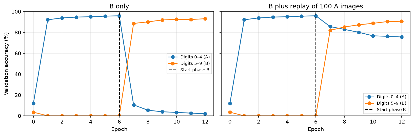
After phase B, what do you predict will happen to accuracy on digits 0–4?

What happened to the earlier classes?

Test accuracy in the recorded MNIST run:

Checkpoint Digits 0–4 (A) Digits 5–9 (B)
After A 97.0% 0.0%
After B only 2.3% 93.8%

Which examples were absent from phase B? How could we put some of that information back?

Catastrophic forgetting: further training can sharply reduce performance on earlier tasks.

Could a small memory help?

What would change if some phase-B updates also included earlier examples?

Epilogue

Summary

  • Optimization: a correct local gradient does not guarantee successful training.
  • Gradient propagation: activation choice, initialization, clipping, and update size address different difficulties.
  • Outputs and losses: choose the output representation and objective together; distinguish logits, probabilities, and class labels.
  • Generalization: L1/L2, dropout, and early stopping can help; evaluate their strength with validation data.
  • Retention: further training can cause forgetting; evaluate old capabilities and consider mechanisms such as replay.
  • Implementation: SimpleMLP preserves the backpropagation structure while adding training choices.

Next lecture

For images, could an architecture use spatial structure instead of treating every input connection alike?

  • Convolutional neural networks address this architectural question.

References

Géron, Aurélien. 2022. Hands-on Machine Learning with Scikit-Learn, Keras, and TensorFlow. 3rd ed. O’Reilly Media, Inc.
Glorot, Xavier, and Yoshua Bengio. 2010. “Understanding the Difficulty of Training Deep Feedforward Neural Networks.” In Proceedings of the Thirteenth International Conference on Artificial Intelligence and Statistics, edited by Yee Whye Teh and Mike Titterington, vol. 9. Proceedings of Machine Learning Research. PMLR. https://proceedings.mlr.press/v9/glorot10a.html.
Hinton, Geoffrey E., Nitish Srivastava, Alex Krizhevsky, Ilya Sutskever, and Ruslan Salakhutdinov. 2012. “Improving Neural Networks by Preventing Co-Adaptation of Feature Detectors.” CoRR abs/1207.0580. http://arxiv.org/abs/1207.0580.
Krizhevsky, Alex, Ilya Sutskever, and Geoffrey E Hinton. 2012. “ImageNet Classification with Deep Convolutional Neural Networks.” In Advances in Neural Information Processing Systems, edited by F. Pereira, C. J. Burges, L. Bottou, and K. Q. Weinberger, vol. 25. Curran Associates, Inc. https://proceedings.neurips.cc/paper_files/paper/2012/file/c399862d3b9d6b76c8436e924a68c45b-Paper.pdf.
LeCun, Yann, Yoshua Bengio, and Geoffrey Hinton. 2015. “Deep Learning.” Nature 521 (7553): 436–44. https://doi.org/10.1038/nature14539.
Rumelhart, David E., Geoffrey E. Hinton, and Ronald J. Williams. 1986. “Learning representations by back-propagating errors.” Nature 323 (6088): 533–36. https://doi.org/10.1038/323533a0.
Russell, Stuart, and Peter Norvig. 2020. Artificial Intelligence: A Modern Approach. 4th ed. Pearson. http://aima.cs.berkeley.edu/.

Appendix: Extending the implementation

From SimplerMLP to SimpleMLP

Which choices require code changes, and where do they enter the computation?

Component SimplerMLP (Lecture 13) SimpleMLP
Hidden activation Sigmoid Sigmoid or ReLU
Initialization Glorot He for ReLU; Glorot for sigmoid
Output Sigmoid probability Sigmoid probability
Learning rate Constant Constant or exponential decay
Loss Mean BCE Mean BCE plus optional L2
Dropout None Optional; one rate for all hidden layers
Example order Shuffle every epoch Optional shuffling (default: on)
Forward caches Activations and preactivations Also scaled dropout masks
Prediction and training API Same methods Same methods

SimpleMLP

Show code
import numpy as np

def sigmoid(z):
    return 1.0 / (1.0 + np.exp(-z))

def sigmoid_prime(z):
    a = sigmoid(z)
    return a * (1.0 - a)

def bce_loss(y_true, y_prob, eps=1e-9):
    """Binary cross-entropy averaged over examples."""
    p = np.clip(y_prob, eps, 1 - eps)
    return -np.mean(y_true * np.log(p) + (1 - y_true) * np.log(1 - p))

def xavier_init(rng, fan_in, fan_out):
    std = np.sqrt(2.0 / (fan_in + fan_out))
    return rng.normal(0.0, std, size=(fan_in, fan_out))

def relu(z):
    return np.maximum(0.0, z)

def relu_prime(z):
    return (z > 0).astype(float)

def he_init(rng, fan_in, fan_out):
    std = np.sqrt(2.0 / fan_in)
    return rng.normal(0.0, std, size=(fan_in, fan_out))

class SimpleMLP:
    """Binary MLP with hidden activation choice, L2, dropout, and LR decay."""

    def __init__(self, layer_sizes, lr=0.1, seed=None, l2=0.0,
                 hidden_activation="relu", lr_decay=None, dropout_rate=0.0):
        self.sizes = list(layer_sizes)
        self.lr = float(lr)
        self.base_lr = float(lr)
        self.l2 = float(l2)
        self.hidden_activation = hidden_activation
        self.lr_decay = lr_decay
        self.dropout_rate = float(dropout_rate)
        self.rng = np.random.default_rng(seed)

        self.W = []
        L = len(self.sizes) - 1
        for l, (din, dout) in enumerate(zip(self.sizes[:-1], self.sizes[1:]), start=1):
            if l < L and self.hidden_activation == "relu":
                Wk = he_init(self.rng, din, dout)
            else:
                Wk = xavier_init(self.rng, din, dout)
            self.W.append(Wk)
        self.b = [np.zeros(dout) for dout in self.sizes[1:]]

    def _act(self, z, last=False):
        if last:
            return sigmoid(z)
        return relu(z) if self.hidden_activation == "relu" else sigmoid(z)

    def _act_prime(self, z, last=False):
        if last:
            return sigmoid_prime(z)
        return relu_prime(z) if self.hidden_activation == "relu" else sigmoid_prime(z)

    def forward(self, X):
        a = X
        L = len(self.W)
        for l, (W, b) in enumerate(zip(self.W, self.b), start=1):
            a = self._act(a @ W + b, last=(l == L))
        return a.ravel()

    def predict_proba(self, X):
        return self.forward(X)

    def predict(self, X, threshold=0.5):
        return (self.predict_proba(X) >= threshold).astype(int)

    def loss(self, X, y):
        """Report mean BCE plus L2 with dropout disabled."""
        p = self.predict_proba(X)
        base = bce_loss(y, p)
        if self.l2 > 0:
            base += 0.5 * self.l2 * sum((W ** 2).sum() for W in self.W)
        return base

    def _forward_full(self, X):
        a = X
        activations = [a]
        zs = []
        dropout_masks = []
        L = len(self.W)
        for l, (W, b) in enumerate(zip(self.W, self.b), start=1):
            z = a @ W + b
            a = self._act(z, last=(l == L))

            # Identity mask for the output layer and when dropout is disabled.
            mask = np.ones_like(a)
            if l < L and self.dropout_rate > 0:
                keep_prob = 1.0 - self.dropout_rate
                mask = (self.rng.random(a.shape) >= self.dropout_rate) / keep_prob
                a = a * mask

            zs.append(z)
            activations.append(a)
            dropout_masks.append(mask)
        return activations, zs, dropout_masks

    def train(self, X, y, epochs=30, batch_size=None, verbose=True, shuffle=True):
        """X: (N, d), y: (N,); batch_size=None uses the full dataset."""
        N = X.shape[0]
        idx = np.arange(N)
        B = N if batch_size is None else int(batch_size)

        for ep in range(1, epochs + 1):
            if shuffle:
                self.rng.shuffle(idx)
            if self.lr_decay is not None:
                self.lr = self.base_lr * self.lr_decay ** (ep - 1)

            base_loss = self.loss(X, y)

            for start in range(0, N, B):
                sl = idx[start:start + B]
                Xb = X[sl]
                yb = y[sl].reshape(-1, 1)
                Bsz = Xb.shape[0]

                activations, zs, dropout_masks = self._forward_full(Xb)
                A_L = activations[-1]

                # Each row is a single example's preactivation sensitivity.
                delta = A_L - yb
                grads_W = [None] * len(self.W)
                grads_b = [None] * len(self.b)

                # Average parameter gradients over examples exactly once.
                grads_W[-1] = activations[-2].T @ delta / Bsz
                grads_b[-1] = delta.mean(axis=0)

                for k in range(len(self.W) - 2, -1, -1):
                    z = zs[k]
                    d_act = self._act_prime(z, last=False)
                    delta = delta @ self.W[k + 1].T
                    delta = delta * dropout_masks[k]
                    delta = delta * d_act
                    grads_W[k] = activations[k].T @ delta / Bsz
                    grads_b[k] = delta.mean(axis=0)

                if self.l2 > 0:
                    for k in range(len(self.W)):
                        grads_W[k] += self.l2 * self.W[k]

                # All gradients use the weights from the same forward pass.
                for k in range(len(self.W)):
                    self.W[k] -= self.lr * grads_W[k]
                    self.b[k] -= self.lr * grads_b[k]

            new_loss = self.loss(X, y)
            if verbose:
                print(f"Epoch {ep:3d} | loss {base_loss:.5f} -> {new_loss:.5f} | lr={self.lr:.4f}")
Choosing hidden activations

If the forward activation changes, which local derivative must the backward pass use?

    def _act(self, z, last=False):
        if last:
            return sigmoid(z)
        return relu(z) if self.hidden_activation == "relu" else sigmoid(z)

    def _act_prime(self, z, last=False):
        if last:
            return sigmoid_prime(z)
        return relu_prime(z) if self.hidden_activation == "relu" else sigmoid_prime(z)

L2 in the objective and gradient

J_{\mathrm{reg}}=J_{\mathrm{BCE}}+ \frac{\lambda}{2}\sum_{l=1}^{L}\|W^{(l)}\|_F^2.

base += 0.5 * self.l2 * sum((W ** 2).sum() for W in self.W)

# After computing the mean data-loss gradients:
grads_W[k] += self.l2 * self.W[k]

Dropout in the forward and backward passes

What extra local derivative does dropout introduce?

During the training forward pass, for a hidden layer:

keep_prob = 1.0 - self.dropout_rate
mask = (self.rng.random(a.shape) >= self.dropout_rate) / keep_prob
a = a * mask

During the backward pass, reuse the cached scaled mask:

delta = delta * dropout_masks[k]

Enable with dropout_rate=0.2; the default of zero disables dropout.

Same API, extended model

from sklearn.datasets import make_circles
from sklearn.model_selection import train_test_split
from sklearn.preprocessing import StandardScaler
from sklearn.metrics import accuracy_score

X, y = make_circles(n_samples=200, factor=0.5, noise=0.08, random_state=1)
X_train, X_test, y_train, y_test = train_test_split(
    X, y, test_size=0.3, random_state=0, stratify=y)

scaler = StandardScaler()
X_train = scaler.fit_transform(X_train)
X_test = scaler.transform(X_test)

model = SimpleMLP([2, 4, 4, 1], lr=0.3, seed=42,
                  hidden_activation="relu", l2=0.001, lr_decay=0.995)
model.train(X_train, y_train, epochs=500, batch_size=32, verbose=False)

print("Train acc:", accuracy_score(y_train, model.predict(X_train)))
print(" Test acc:", accuracy_score(y_test, model.predict(X_test)))
Train acc: 1.0
 Test acc: 1.0

Computing softmax safely

Subtracting the largest logit preserves the probabilities and avoids exponentiating large positive values.

Show code
import numpy as np

logits = np.array([1000.0, 1001.0, 999.0])
exp_scores = np.exp(logits-logits.max())
probabilities = exp_scores/exp_scores.sum()
print('Probabilities:', probabilities.round(4))
print('Sum:', probabilities.sum())
Probabilities: [0.2447 0.6652 0.09  ]
Sum: 0.9999999999999999

Marcel Turcotte

Marcel.Turcotte@uOttawa.ca

School of Electrical Engineering and Computer Science (EECS)

University of Ottawa