Introduction to machine learning

CSI 4106 - Fall 2026

Marcel Turcotte

Version: Sep 15, 2026 11:59

Preamble

Message of the day (1/2)

The AI Researcher Who Just Quit Anthropic Says It’s ‘Crunch Time for Humanity’. Wired. 2026-09-09.

Message of the day (2/2)

Why Do We Tell Ourselves Scary Stories About AI?. Quanta Magazine, 2026-04-10.

From the Previous Lecture

• Symbolic and connectionist methods are two major traditions in AI.
• Defining intelligence remains challenging.
• Russell and Norvig describe four perspectives on AI: thinking humanly, acting humanly, thinking rationally, and acting rationally.
• Narrow AI targets particular tasks; artificial general intelligence is a broader and contested goal.
• Difficult, unresolved questions frequently concern embodiment, agency, sentience, consciousness, emotion, and cognition.

Learning objectives

• Distinguish supervised, unsupervised, and reinforcement learning by the feedback available
• Identify examples, features, and targets in a supervised-learning dataset
• Differentiate classification from regression, and learning from inference
• Apply the basic scikit-learn workflow: load data, explore it, fit a model, and make predictions
• Explain why a separate test set is needed to estimate performance on unseen data

Reading: Russell and Norvig (2020), Chapter 19, “Learning from Examples.”

Introduction

Rationale

Why should a computer program learn?

1. Adaptability and Continuous Improvement:
   • Adaptability to Dynamic Environments: Programs that learn can adapt to changing conditions, remaining effective in dynamic settings.
     • Example: Self-driving cars adjusting to traffic and weather changes.
   • Continuous Improvement: Learning enables systems to stay current with new data and trends without constant human intervention.
     • Example: Spam filters evolving to counter new spam techniques.
2. Enhanced Performance and Efficiency:
   • Improved Performance: Learning allows programs to improve their performance based on past experience or data.
     • Example: Recommendation systems refining suggestions with more user data.
   • Cost-Effectiveness: Automating the learning process reduces the need for manual updates, leading to cost savings.
     • Example: Predictive maintenance systems minimizing manual inspections.
3. Complex Problem Solving and Hidden Pattern Discovery:
   • Handling Complex Problems: Learning algorithms tackle problems that are too intricate for static, rule-based systems.
     • Example: Image recognition distinguishing between different objects.
   • Discovering Hidden Patterns: Learning models can uncover relationships in data that are not evident to human analysts.
     • Example: Identifying complex genomic relationships in bioinformatics.
4. Personalization and Scalability:
   • Personalization: Learning allows programs to provide tailored outputs to individual users, enhancing the user experience.
     • Example: Virtual assistants learning user preferences.
   • Scalability: Learning algorithms efficiently manage and analyze large datasets, improving their utility.
     • Example: Search engines optimizing result relevance with machine learning.
5. Innovation and Research:
   • Fostering Innovation: Learning algorithms can simulate new ideas, leading to advancements and discoveries.
     • Example: Machine learning models predicting drug efficacy in pharmaceutical research.

Attribution: Gemini 1.5 Flash, Aug. 14, 2024, prompted with “In the style of a children’s book, create the image of a cute robot holding a red flower.”

Definition

Mitchell (1997), page 2

A computer program is said to learn from experience E with respect to some class of tasks T and performance measure P, if its performance at tasks in T, as measured by P, improves with experience E.

Although this book was published in 1997, it has been influential and remains relevant. Unlike many other machine learning books, it is particularly engaging.

This particular definition of learning is often reused.

Tom M Mitchell. Machine Learning. McGraw-Hill, New York, 1997. (PDF)

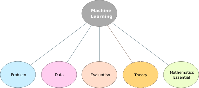
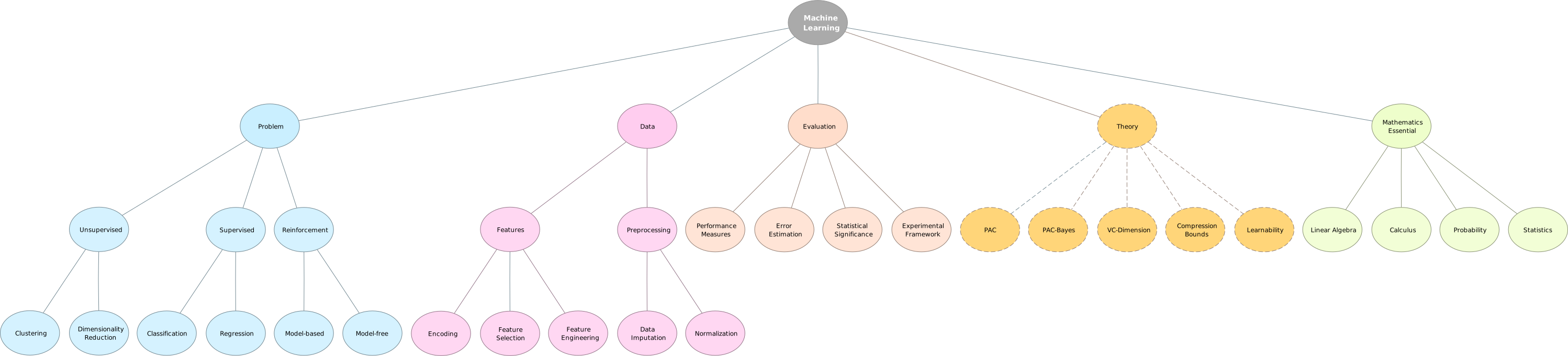
Concepts

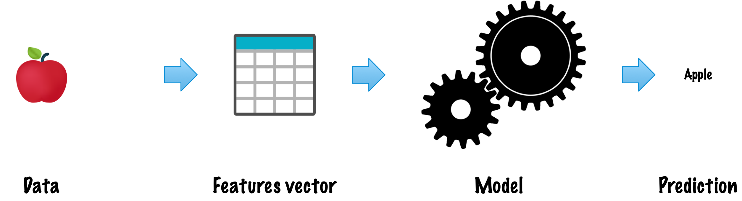
See: ml_concepts-00.svg

Types of problems

We will begin with three broad learning settings, distinguished by the feedback available:

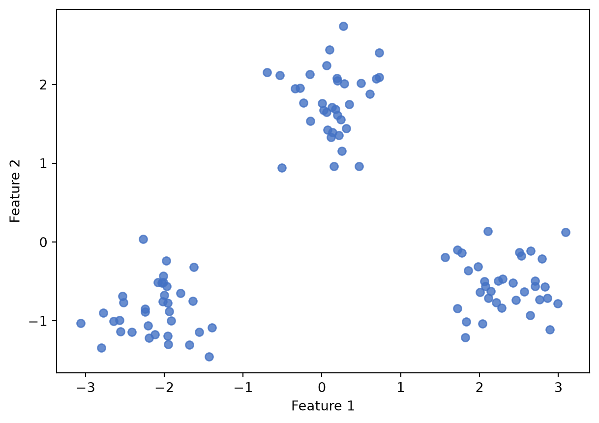
1. Unsupervised learning: The examples have no target labels.
2. Supervised learning: Each training example is accompanied by a target label.
3. Reinforcement learning: An agent receives numerical rewards while interacting with an environment.

Supervised learning is the most extensively studied and arguably the most intuitive type of learning. It is typically the first type of learning introduced in educational contexts.

Unsupervised Learning

Given: feature vectors x_1, x_2, \ldots, x_N, but no target labels y_i.

import matplotlib.pyplot as plt
import numpy as np

rng = np.random.default_rng(7)
centres = [(-2.0, -0.8), (0.2, 1.8), (2.3, -0.5)]
points = np.vstack([
    rng.normal(loc=centre, scale=0.42, size=(35, 2))
    for centre in centres
])

plt.scatter(points[:, 0], points[:, 1], color="#4472C4", alpha=0.8)
plt.xlabel("Feature 1")
plt.ylabel("Feature 2")
plt.gca().set_aspect("equal", adjustable="box")
plt.show()

Every point has the same colour because no class labels were supplied. A clustering algorithm attempts to infer groups from the feature values.

In unsupervised learning, an algorithm receives examples without target labels and attempts to discover useful structure in them.

Clustering groups examples that are similar according to the selected features and distance measure. The groups are inferred rather than supplied by a teacher. They should not automatically be interpreted as objectively correct or meaningful categories: the result can change with the features, scaling, algorithm, and its settings.

Other unsupervised-learning tasks include:

• dimensionality reduction, which represents data using fewer variables while preserving useful structure;
• density estimation, which models where observations tend to occur; and
• anomaly detection, which identifies observations that differ markedly from the usual patterns.

This course will not develop these methods further; the objective here is to recognize the paradigm and distinguish it from supervised learning.

Finding structure without labels

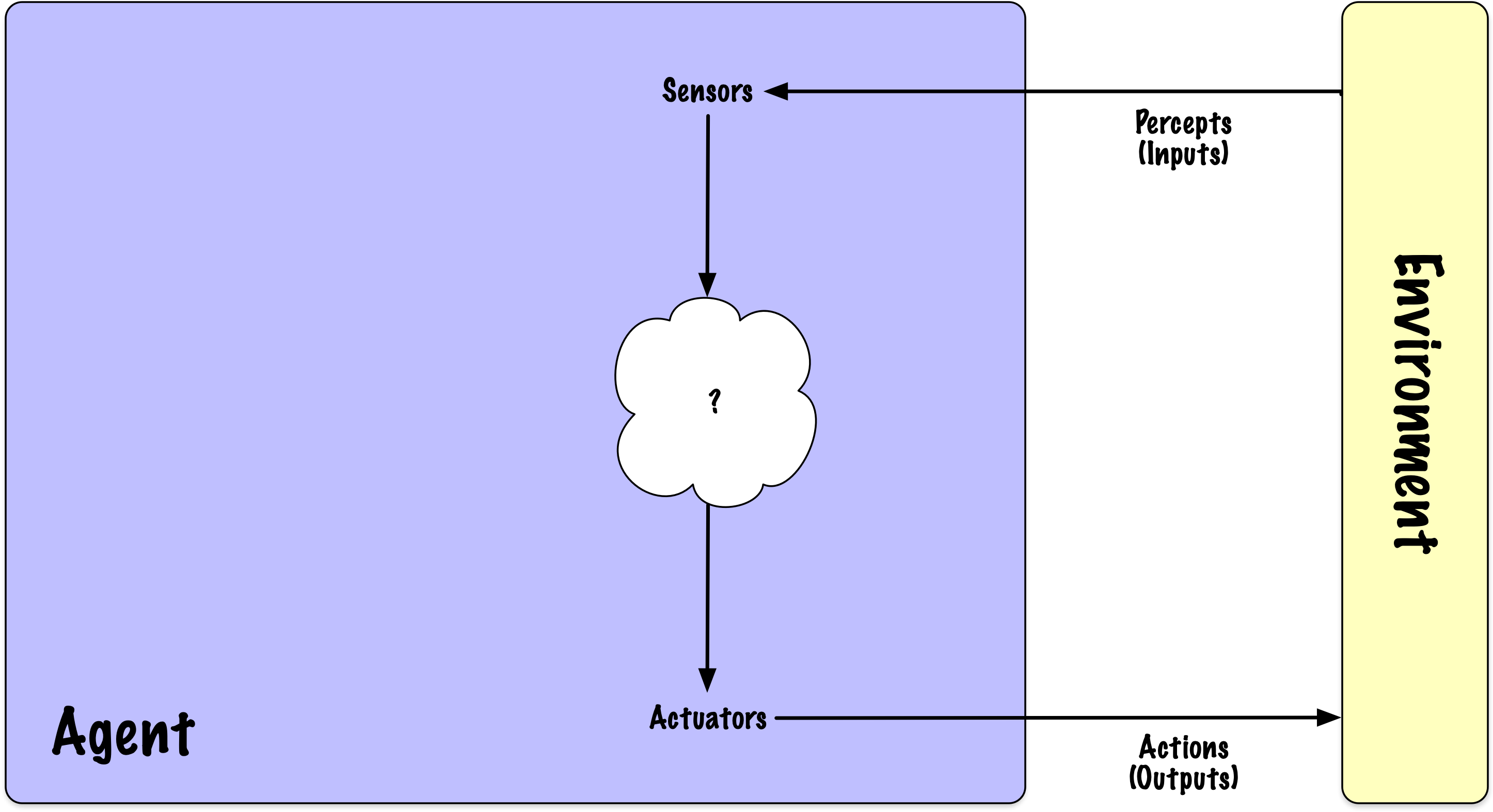
Reinforcement Learning

An agent takes actions in an environment, observes the consequences, and receives numerical rewards.

Goal: Learn a policy for choosing actions that maximizes cumulative reward.

In reinforcement learning, an agent learns through repeated interaction with an environment. At each step, it receives an observation, chooses an action, and receives a numerical reward together with the next observation.

The reward evaluates the consequences of behaviour, but it is not a target label specifying the correct action. Rewards may also be delayed: an action can affect outcomes many steps later. The agent must therefore learn a policy—a strategy for choosing actions—that performs well over time rather than merely maximizing the immediate reward.

Typical applications include games, robotics, resource allocation, and control systems. A central difficulty is balancing exploration of unfamiliar actions with exploitation of actions that have worked well so far.

This course will not develop reinforcement-learning algorithms further; students should be able to identify the agent, environment, actions, observations, rewards, and overall objective.

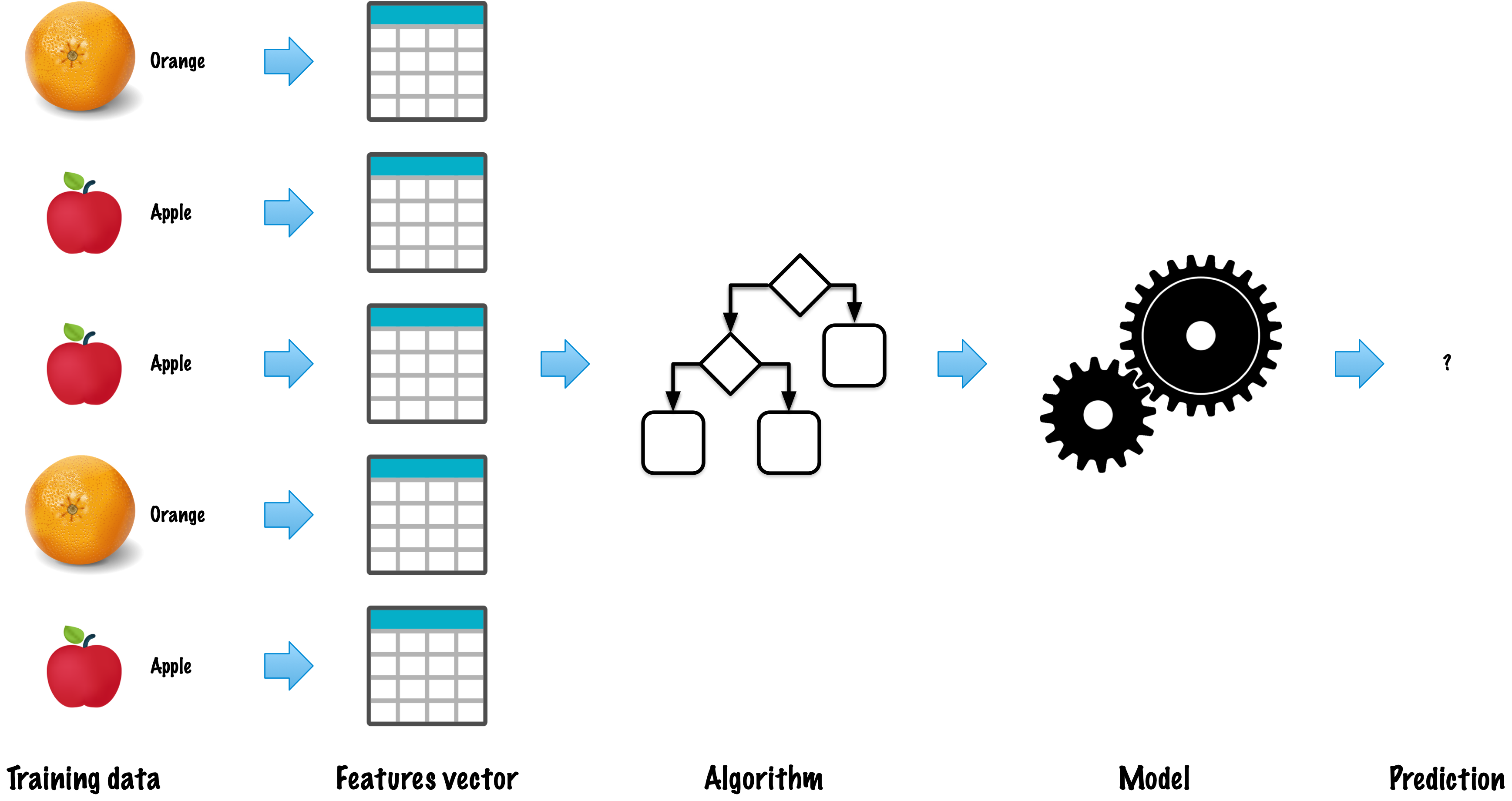
Supervised Learning: Two Phases

For the supervised-learning workflow studied in this course:

1. Learning (building a model)
2. Inference (using the model)

Separating learning from inference is a useful description of the batch supervised-learning workflow used in this course. It is not universal: in reinforcement learning, for example, acting, receiving feedback, and updating the policy may be interleaved.

Learning: Building a Model

In machine learning, the learning phase is often the most challenging and resource-intensive component. This stage necessitates meticulous attention to data curation, as well as the selection and training of an appropriate algorithm.

Training some contemporary frontier models is estimated to cost more than US$100 million.

Source: Stanford University Human-Centered Artificial Intelligence 2025 AI Index Report

Developing such models necessitates infrastructure investments that could reach trillions of dollars.

• “By the end of 2024, we’re aiming to continue to grow our infrastructure build-out that will include 350,000 NVIDIA H100 GPUs as part of a portfolio that will feature compute power equivalent to nearly 600,000 H100s.”
  • Building Meta’s GenAI Infrastructure, 2024-03-12.
• OpenAI’s Sam Altman Expects to Spend ‘Trillions’ on Infrastructure, Bloomberg, 2025-08-15.

Inference: Using a Model

Inference for one example typically demands fewer computational resources than training a model. However, the total cost can still be substantial when a model serves many users, and some reasoning systems deliberately use more computation at inference time.

• OpenAI’s o3 Reasoning Models Are Extremely Expensive to Run, Alexandra Tremayne-Pengelly, Observer, 2025-04-04. Media cost estimates depend strongly on the inference configuration and should not be interpreted as a stable price per query.

Carp-e Diem! (example)

1. Problem: Will They Bite Today?

Objective: Develop a predictive model that classifies a fishing day as Poor, Average, or Excellent.

Supervised learning involves training a model on labelled data so that it can make predictions on new, unseen data.

The specific task is classification.

“Poor”, “Average”, and “Excellent” are classes (for the target variable).

Attribution: Gemini 1.5 Flash, Sept. 10, 2024, prompted with “In the style of a children’s book, generate the image of a fish with a farmer’s hat.”

2. Attributes (features)

Fishing traditions and guides, including The Old Farmer’s Almanac, often use the moon phase when recommending fishing days. We will treat it as a candidate feature; whether it is genuinely predictive is an empirical question.

• Moon Phase (Categorical): ‘New Moon’, ‘First Quarter’, ‘Full Moon’, and ‘Last Quarter’.
• Forecast (Categorical): ‘Rainy’, ‘Cloudy’, and ‘Sunny’.
• Outdoor Temperature (Numerical): The air temperature in degrees Celsius.
• Water Temperature (Numerical): The water temperature of the lake or river.

Obviously, real-world applications will have many more attributes.

3. Training data

Example	Moon Phase	Forecast	Outdoor Temperature (°C)	Water Temperature (°C)	Fishing Outcome
1	Full Moon	Sunny	25	22	Excellent
2	New Moon	Cloudy	18	19	Average
3	First Quarter	Rainy	15	17	Poor
4	Last Quarter	Sunny	30	24	Excellent
5	Full Moon	Cloudy	20	20	Average
6	New Moon	Rainy	22	21	Poor

This is a supervised-learning problem because the target is known for each training example. Since the possible targets are categories, it is a classification task.

This small dataset is invented for illustration. It contains only six examples; a real study would require substantially more representative observations and a carefully defined outcome.

The choice of attributes and the quality of the data are crucial to model performance. An attribute such as the colour of your socks is unlikely to have much effect on the predictions.

Therefore, a machine learning project typically begins with an exploratory phase, which involves analyzing the data, examining distributions, and identifying correlations.

3. Training data: data representation

Moon Phase	Forecast	Outdoor Temperature (°C)	Water Temperature (°C)
Full Moon	Sunny	25	22
New Moon	Cloudy	18	19
First Quarter	Rainy	15	17
Last Quarter	Sunny	30	24
Full Moon	Cloudy	20	20
New Moon	Rainy	22	21

The data is often presented in a tabular (matrix) format, where each row represents an attribute vector (feature vector), typically denoted as x_i, which corresponds to the i-th example in the training set.

3. Training data: label representation

Fishing Outcome
Excellent
Average
Poor
Excellent
Average
Poor

The labels are generally represented as a column vector, with y_i denoting the label for the i-th example.

4. Model Training

Model training uses labelled examples to construct a model that can make predictions. Depending on the algorithm, training may estimate parameters, build a structure, or simply store examples.

4. Model Training (continued)

A simple model that fits all six training examples is:

• If the forecast is Sunny, predict Excellent.
• If the forecast is Cloudy, predict Average.
• If the forecast is Rainy, predict Poor.

Fitting six examples does not establish that the model will predict new fishing days accurately.

5. Prediction

Given new, unseen data, predict today’s fishing category.

• Moon Phase: New Moon
• Forecast: Sunny
• Outdoor Temperature: 24°C
• Water Temperature: 21°C

Prediction: Excellent

Life cycle

1. Data collection and preparation
2. Feature engineering
3. Training
4. Model evaluation
5. Model deployment
6. Monitoring and maintenance

• Data collection and preparation are critical and labor-intensive processes.
  • There must be sufficient data.
  • The data must be of high quality; for instance, it should not be excessively noisy.
  • There should be few missing values.
  • Most importantly, the data should be representative. We expect that new data will be generated from the same process and have the same distribution.
    • The importance of this cannot be overstated.
      • Consider image classification software that was not trained on a diverse sample in terms of ethnicity, gender, body size, or social status.
      • Think of medical applications and the consequences of datasets that are not sufficiently diverse.
• Feature engineering is the process of selecting, transforming, and creating input variables (features) that make useful patterns easier for a model to learn. It can include scaling numerical variables, representing categorical variables, and constructing new features.
  • Deep learning can learn useful representations directly from data, but data preparation and feature choices remain important.
• Model evaluation is the process of assessing a machine learning model’s performance using specific metrics, such as accuracy, precision, recall, F1-score, or AUC-ROC. This typically involves testing the model on a separate validation or test dataset to ensure it generalizes well to unseen data and meets the desired criteria for accuracy and reliability.
• Model deployment: The trained model is integrated into an application. Many deployed models have fixed parameters and are updated periodically; others learn continuously from new data. The appropriate strategy depends on cost, risk, and how quickly the data-generating process changes.
• Monitoring and maintenance: The performance of the model needs to be continuously monitored. Concept drift is often observed, requiring the system to be retrained. Spam detection is a good example. Once the system is deployed, spammers adapt and find ways to circumvent the spam detection mechanisms put in place.

Formal definitions

Supervised learning (notation)

The dataset (“experience”) is a collection of labelled examples.

• \{(x_i, y_i)\}_{i=1}^N
  • Each x_i is a feature (attribute) vector with D dimensions.
  • x_i^{(j)} is the value of feature j for example i, where j \in \{1, \ldots, D\} and i \in \{1, \ldots, N\}.
  • The target y_i may be a class from a finite set \{1, 2, \ldots, C\}, a real number, or a structured object such as a sequence, tree, or graph.

Problem: Given the dataset, create a model that can predict the value of y for an unseen x.

This notation follows that of The Hundred-Page Machine Learning Book by Andriy Burkov.

Supervised learning (notation, continued)

• When the target y_i is a class, taken from a finite list of classes, \{1, 2, \ldots, C\}, we call the task a classification task.

• When the target y_i is a real number, we call the task a regression task.

Anil Ananthaswamy, in his book Why Machines Learn: The Elegant Math Behind Modern AI, offers an example inspired by the COVID-19 pandemic.

In this advanced scenario, hospitals globally are systematically compiling patient data from the early stages of the COVID-19 pandemic. Each patient is characterized by six key variables: x_1 representing age, x_2 indicating body mass index, x_3 denoting difficulty breathing (encoded as 1 for yes and 0 for no), x_4 signifying the presence of fever (yes/no), x_5 for diabetes status (yes/no), and x_6 describing chest CT scan results (0 for clear, 1 for mild infection, 2 for severe infection). These variables collectively form a six-dimensional vector for each patient.

Clinicians have observed that patients typically follow one of two trajectories: they either stabilize and are discharged approximately three days after admission, or their condition deteriorates, necessitating ventilator support. Consequently, each patient is assigned an outcome variable, y, where y = -1 indicates no need for ventilator support after three days, and y = 1 indicates the requirement for ventilator support after three days.

Can you think of examples of regression tasks? The defining feature is that the target is a numerical quantity. Examples include:

• estimating the selling price of a house;
• forecasting tomorrow’s temperature or electricity demand;
• estimating travel time or remaining battery life;
• predicting medical costs; and
• estimating the amount a customer will spend.

Some problems can be formulated in more than one way. Predicting whether a borrower will default is classification; predicting the probability of default produces a numerical score.

Example with code

Scikit-learn

scikit-learn.org

scikit-learn is an open-source machine learning library that supports supervised and unsupervised learning. It also provides tools for model fitting, data preprocessing, model selection, model evaluation, and many other tasks.

scikit-learn provides dozens of built-in machine learning algorithms and models, called estimators.

Built on NumPy, SciPy, and matplotlib.

We will use scikit-learn for this example and throughout the coming weeks.

Scikit-learn

Attribution: Choosing the right estimator

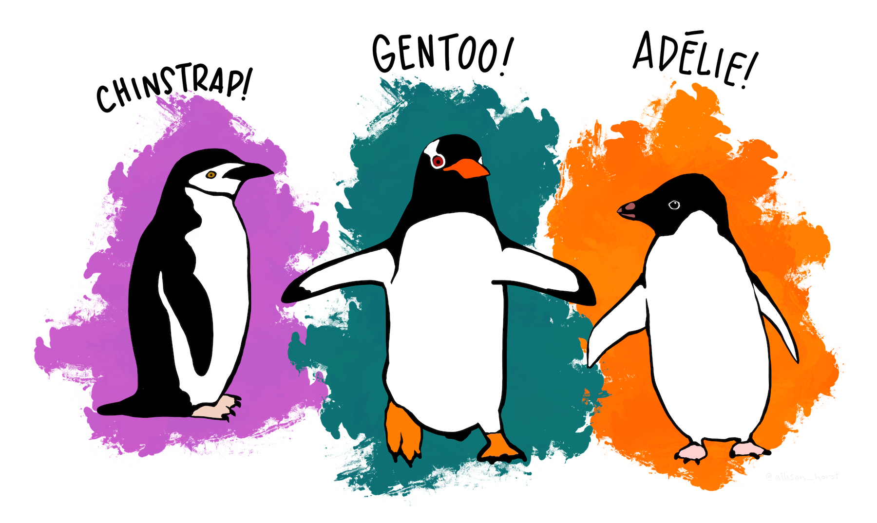
Example: Palmer Penguins Dataset

The Palmer penguins dataset by Allison Horst, Alison Hill, and Kristen Gorman was first made publicly available as an R package. The goal of the Palmer Penguins dataset is to replace the highly overused Iris dataset for data exploration & visualization.

Using this Python package you can easily load the Palmer penguins into your Python environment.

Initially, we will examine the entire example from a high-level perspective to provide a clear overview of the steps involved. Subsequently, we will revisit this example in greater detail.

The Palmer penguins dataset by Allison Horst, Alison Hill, and Kristen Gorman. Artwork by @allison_horst

Example: In Case of a Missing Library

try:
    from palmerpenguins import load_penguins
except ModuleNotFoundError:
    %pip install -q palmerpenguins
    from palmerpenguins import load_penguins

If you are executing this Jupyter Notebook within Google Colab or any environment where the library is not pre-installed, proceed with the installation.

Example: Loading the Data

# It is customary to use X and y for the data and labels

X, y = load_penguins(return_X_y = True)

# Remove rows with missing measurements

X = X.dropna()
y = y.loc[X.index]

Two penguins have missing measurements. For this first example, we remove those rows before training.

Example: Using a Decision Tree

from sklearn import tree

clf = tree.DecisionTreeClassifier(criterion="entropy", random_state=42)

Available classifiers include decision trees, support vector machines, k-nearest neighbours, logistic regression, and neural networks.

Example: Training

# Training

clf = clf.fit(X, y)

scikit-learn estimators share a consistent interface. Classifiers expose methods such as fit, predict, and score.

The DecisionTreeClassifier in scikit-learn constructs a decision tree by recursively splitting the dataset. With criterion="entropy", it selects thresholds that produce the greatest reduction in weighted entropy. Here is a concise description of the process:

1. Initialization: The algorithm starts with the entire dataset as the root node.

2. Splitting criterion: At each node, it evaluates candidate thresholds across the available numerical features and retains the split that best separates the classes.

3. Recursive Splitting: The dataset is divided into subsets based on the selected attribute and threshold, creating child nodes. This process is repeated recursively for each child node.

4. Stopping conditions: Splitting stops when a stopping rule is reached—for example, when a node is pure, no candidate split improves the objective, or a depth or sample-size limit applies.

5. Terminal Nodes: Once splitting is complete, each terminal node is assigned a class label based on the majority class of the samples in that node.

The resulting tree can then be used to classify new samples by traversing from the root to a terminal node, following the decision rules defined at each node.

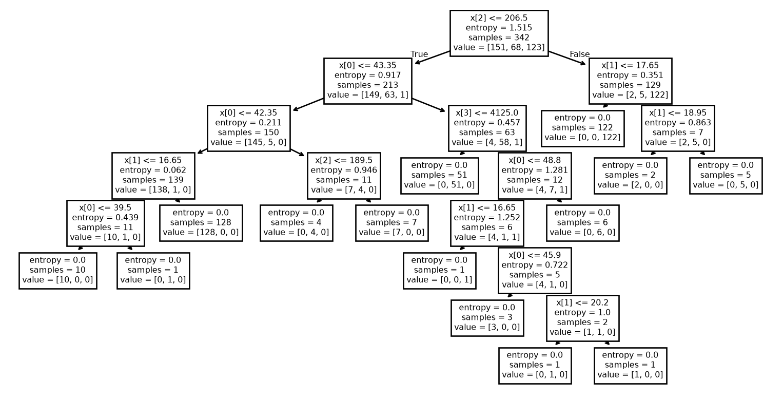
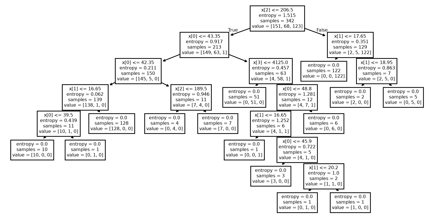
Example: Visualizing the tree (1/2)

import matplotlib.pyplot as plt

tree.plot_tree(clf)
plt.show()

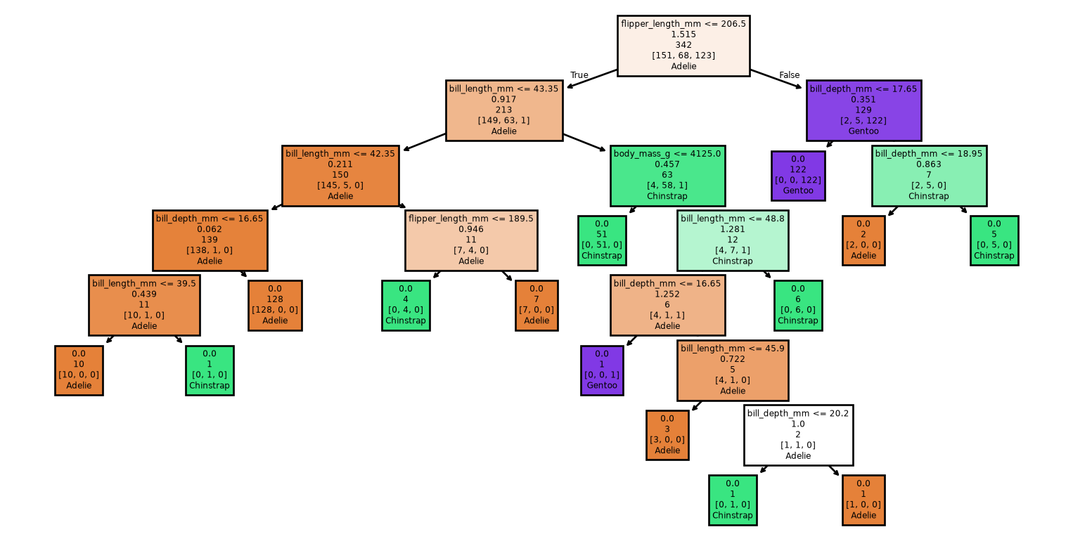
Example: Visualizing the tree (2/2)

target_names = clf.classes_

tree.plot_tree(clf, 
               feature_names = X.columns,
               class_names = target_names,
               label = 'none',
               filled = True)
plt.show()

Example: Prediction

import pandas as pd

# Create two new examples

column_names = ['bill_length_mm', 'bill_depth_mm', 'flipper_length_mm', 'body_mass_g']
new_penguins = pd.DataFrame(
    [[34.2, 17.9, 186.8, 2945.0], [51.0, 15.2, 223.7, 5560.0]],
    columns=column_names,
)

# Prediction

predictions = clf.predict(new_penguins)

# Printing the predicted labels for our two examples

print(predictions)

['Adelie' 'Gentoo']

Example: Complete

X, y = load_penguins(return_X_y = True)
X = X.dropna()
y = y.loc[X.index]
clf = tree.DecisionTreeClassifier(criterion="entropy", random_state=42)
clf = clf.fit(X, y)
tree.plot_tree(clf)
new_penguins = pd.DataFrame(
    [[34.2, 17.9, 186.8, 2945.0], [51.0, 15.2, 223.7, 5560.0]],
    columns=column_names,
)
print(clf.predict(new_penguins))

['Adelie' 'Gentoo']

Example: Apparent Performance

from sklearn.metrics import classification_report, accuracy_score

# Make predictions

y_pred = clf.predict(X)

# Evaluate the model

accuracy = accuracy_score(y, y_pred)
report = classification_report(y, y_pred, labels=clf.classes_, target_names=clf.classes_)

print(f'Accuracy: {accuracy:.2f}')
print('Classification Report:')
print(report)

Example: Apparent Performance

Accuracy: 1.00
Classification Report:
              precision    recall  f1-score   support

      Adelie       1.00      1.00      1.00       151
   Chinstrap       1.00      1.00      1.00        68
      Gentoo       1.00      1.00      1.00       123

    accuracy                           1.00       342
   macro avg       1.00      1.00      1.00       342
weighted avg       1.00      1.00      1.00       342

Example: Discussion

We have demonstrated a complete example:

• Loading the data
• Selecting a classifier
• Training the model
• Visualizing the model
• Making a prediction

However, several simplifications were made throughout this process.

Example: Wait a Minute!

from sklearn.metrics import classification_report, accuracy_score

# Make predictions

y_pred = clf.predict(X)

# Evaluate the model

accuracy = accuracy_score(y, y_pred)
report = classification_report(y, y_pred, labels=clf.classes_, target_names=clf.classes_)

print(f'Accuracy: {accuracy:.2f}')
print('Classification Report:')
print(report)

Important

This example is misleading, or even flawed!

The performance of this classifier appears to be perfect at first glance. However, is it really?

These predictions are made on the same examples used for training. This is training accuracy, not an estimate of performance on unseen data.

Example: Exploration

penguins = load_penguins()

type(penguins)

pandas.DataFrame

penguins.head()

Example: Exploration

	species	island	bill_length_mm	bill_depth_mm	flipper_length_mm	body_mass_g	sex	year
0	Adelie	Torgersen	39.1	18.7	181.0	3750.0	male	2007
1	Adelie	Torgersen	39.5	17.4	186.0	3800.0	female	2007
2	Adelie	Torgersen	40.3	18.0	195.0	3250.0	female	2007
3	Adelie	Torgersen	NaN	NaN	NaN	NaN	NaN	2007
4	Adelie	Torgersen	36.7	19.3	193.0	3450.0	female	2007

Example: Exploration

penguins.describe()

Example: Exploration

	bill_length_mm	bill_depth_mm	flipper_length_mm	body_mass_g	year
count	342.000000	342.000000	342.000000	342.000000	344.000000
mean	43.921930	17.151170	200.915205	4201.754386	2008.029070
std	5.459584	1.974793	14.061714	801.954536	0.818356
min	32.100000	13.100000	172.000000	2700.000000	2007.000000
25%	39.225000	15.600000	190.000000	3550.000000	2007.000000
50%	44.450000	17.300000	197.000000	4050.000000	2008.000000
75%	48.500000	18.700000	213.000000	4750.000000	2009.000000
max	59.600000	21.500000	231.000000	6300.000000	2009.000000

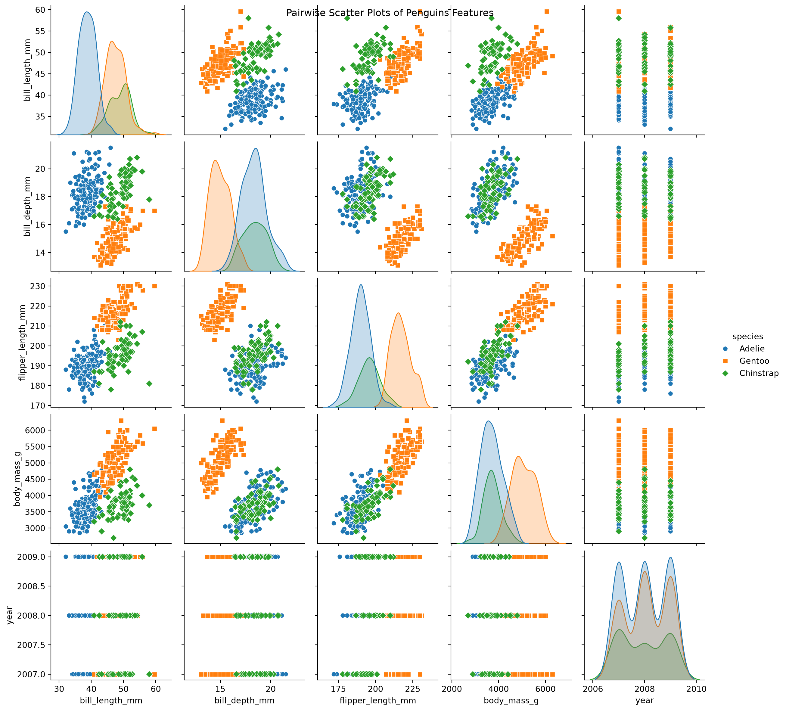
Example: Using Seaborn

import seaborn as sns

# Pairplot using seaborn

sns.pairplot(penguins, hue='species', markers=["o", "s", "D"])
plt.suptitle("Pairwise Scatter Plots of Penguins Features")
plt.show()

What insights can be drawn from examining the graphs?

The figure presents pairwise plots of the Palmer Penguins features, with the diagonal showing the distribution of each individual feature. Each dot represents an example (x), and the colours indicate its label (y).

Let’s first consider the diagonal elements:

• Is it possible to classify the examples using a single feature?
• We observe that each feature alone cannot distinguish between the classes.
• However, plots involving bill depth, body mass, or flipper length help distinguish Gentoo from the other two species, although Adélie and Chinstrap still overlap.

The class Gentoo frequently forms a distinct cluster.

Example: Using Seaborn

Example: Training and Test Set

from sklearn.model_selection import train_test_split

# Split the dataset into training and testing sets

X_train, X_test, y_train, y_test = train_test_split(
    X,
    y,
    test_size=0.2,
    random_state=7,
    stratify=y,
)

We will have a lot more to say about testing in the coming weeks.

For narrative clarity, these slides explored the full dataset before introducing the split. In a rigorous experiment, the test set should be set aside before making data-driven modelling choices and left untouched until final evaluation.

random_state makes the pseudo-random partition reproducible. Changing it changes which examples are held out and may change the measured accuracy. stratify=y keeps the class proportions approximately consistent across the two subsets.

Practice: Experiment with different values for random_state. What do you observe, and why?

Our initial decision tree was constructed and evaluated using the entire dataset. It can fit those examples closely, but this does not tell us how accurately it will predict unseen data.

Example: Creating a New Classifier

clf = tree.DecisionTreeClassifier(criterion="entropy", random_state=42)

Example: Training the New Classifier

clf.fit(X_train, y_train)

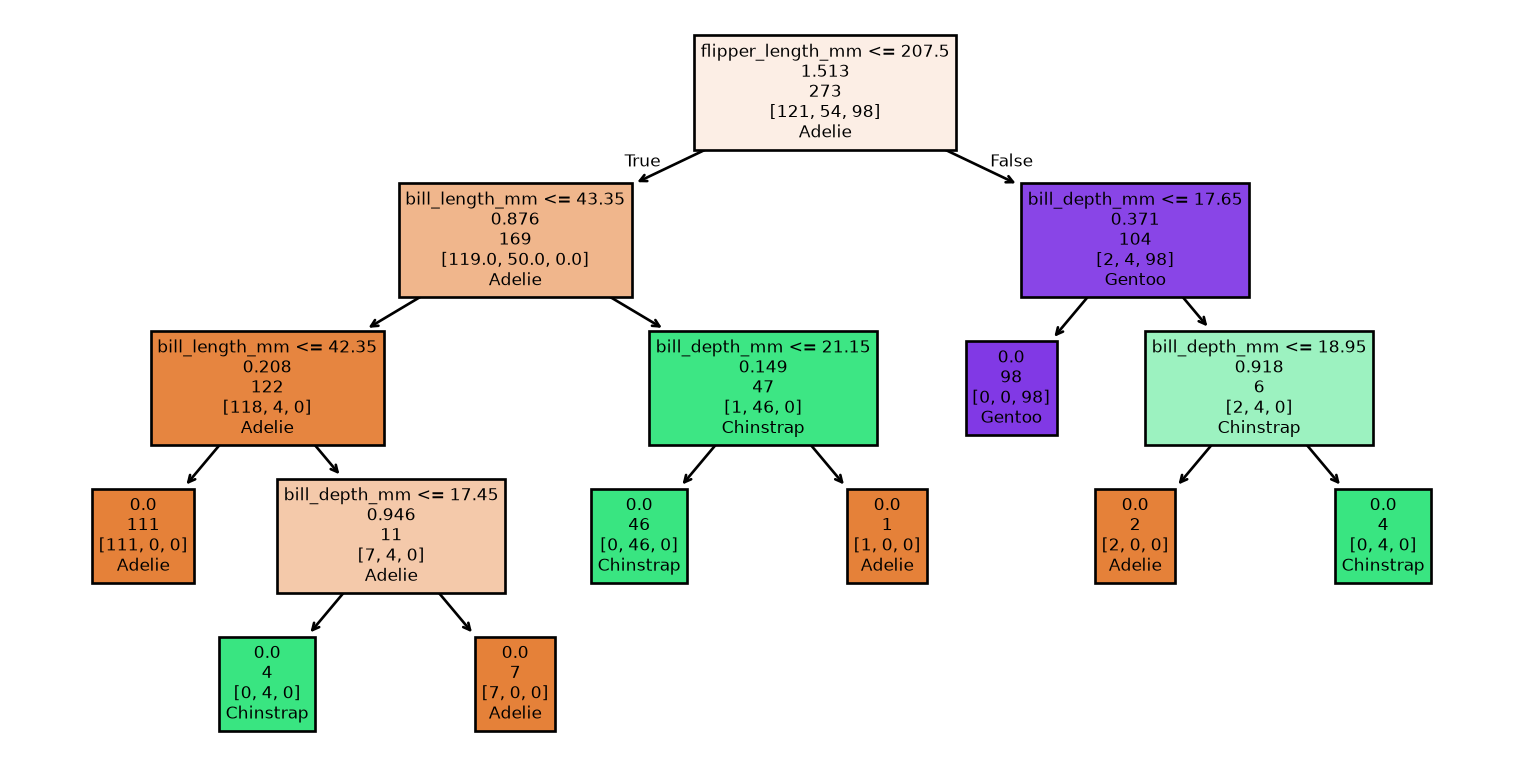
Example: Visualizing the Tree

tree.plot_tree(clf, 
               feature_names = X.columns,
               class_names = target_names,
               label = 'none',
               filled = True)
plt.show()

Example: Making Predictions

# Make predictions
y_pred = clf.predict(X_test)

Example: Measuring the Performance

# Evaluate the model
accuracy = accuracy_score(y_test, y_pred)
report = classification_report(
    y_test,
    y_pred,
    labels=clf.classes_,
    target_names=clf.classes_,
)

print(f'Accuracy: {accuracy:.2f}')
print('Classification Report:')
print(report)

Here is a discussion on model persistence for scikit-learn models.

Example: Measuring the Performance

Accuracy: 0.91
Classification Report:
              precision    recall  f1-score   support

      Adelie       0.96      0.90      0.93        30
   Chinstrap       0.72      0.93      0.81        14
      Gentoo       1.00      0.92      0.96        25

    accuracy                           0.91        69
   macro avg       0.90      0.92      0.90        69
weighted avg       0.93      0.91      0.92        69

Summary

• We distinguished supervised, unsupervised, and reinforcement learning by the feedback available.
• We identified examples, features, and targets in a supervised-learning problem.
• We applied the scikit-learn workflow to the Palmer Penguins dataset.
• We explored the data, trained a classifier, and made predictions.
• We used a separate test set to estimate performance on unseen data.

Prologue

Further readings (1/3)

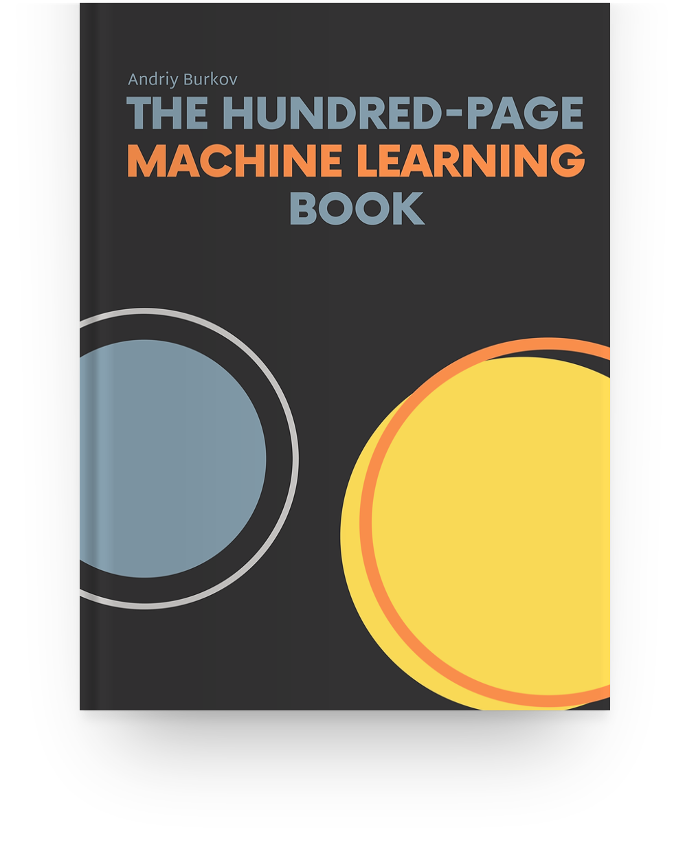
• The Hundred-Page Machine Learning Book (Burkov 2019) is a succinct and focused textbook that can feasibly be read in one week, making it an excellent introductory resource.
• Available under a “read first, buy later” model, allowing readers to evaluate its content before purchasing.
• Its author, Andriy Burkov, received his Ph.D. in AI from Université Laval.

Further readings (2/3)

• Hands-on Machine Learning with Scikit-Learn, Keras, and TensorFlow (Géron 2022) provides practical examples and leverages production-ready Python frameworks.
  • Comprehensive coverage includes not only the models but also libraries for hyperparameter tuning, data preprocessing, and visualization.
  • Code examples and solutions to exercises available as Jupyter Notebooks on GitHub.
  • Aurélien Géron is a former YouTube product manager who led video classification for Search & Discovery.

Further readings (3/3)

• Mathematics for Machine Learning (Deisenroth et al. 2020) aims to provide the necessary mathematical skills to read machine learning books.
• PDF of the book
• “This book provides great coverage of all the basic mathematical concepts for machine learning. I’m looking forward to sharing it with students, colleagues, and anyone interested in building a solid understanding of the fundamentals.” Joelle Pineau, McGill University and Facebook

References

Burkov, Andriy. 2019. The Hundred-Page Machine Learning Book. Andriy Burkov.

Deisenroth, Marc Peter, A. Aldo Faisal, and Cheng Soon Ong. 2020. Mathematics for Machine Learning. Cambridge University Press. https://doi.org/10.1017/9781108679930.

Géron, Aurélien. 2022. Hands-on Machine Learning with Scikit-Learn, Keras, and TensorFlow. 3rd ed. O’Reilly Media, Inc.

Kingsford, C, and Steven L Salzberg. 2008. “What Are Decision Trees?” Nature Biotechnology 26 (9): 1011–13. https://doi.org/10.1038/nbt0908-1011.

Mitchell, Tom M. 1997. Machine Learning. McGraw-Hill.

Russell, Stuart, and Peter Norvig. 2020. Artificial Intelligence: A Modern Approach. 4th ed. Pearson. http://aima.cs.berkeley.edu/.

Next lecture

• Decision trees and entropy
• Decision boundaries and logistic regression
• K-nearest neighbours

Appendix: Iris Dataset

Example: Iris Dataset

Attribution: Diego Mariano, CC BY-SA 4.0, via Wikimedia Commons. See here for information on this dataset.

Example: Loading the Data

from sklearn.datasets import load_iris

# Load the Iris dataset

iris = load_iris()

When using your own dataset, you will generally have to load it from a file or online source, as in the Ottawa River Temperature notebook.

Conveniently, scikit-learn comes with toy and real-world datasets to facilitate experimentation. See here for a description of load_iris.

Example: Using a Decision Tree

from sklearn import tree

clf = tree.DecisionTreeClassifier(criterion="entropy", random_state=42)

Available classifiers include decision trees, support vector machines, k-nearest neighbours, logistic regression, and neural networks.

Example: Training

# It is customary to use X and y for the data and labels

X, y = iris.data, iris.target

# Training

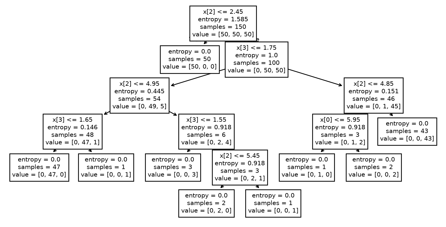
clf = clf.fit(X, y)

scikit-learn estimators share a consistent interface. Classifiers expose methods such as fit, predict, and score.

With criterion="entropy", DecisionTreeClassifier constructs a tree by recursively choosing feature thresholds that reduce weighted entropy. Each split creates two child nodes. Splitting continues until no useful split remains or another stopping condition is reached. Each leaf predicts the majority class among the training examples that reach it.

Example: Visualizing the tree (1/2)

import matplotlib.pyplot as plt

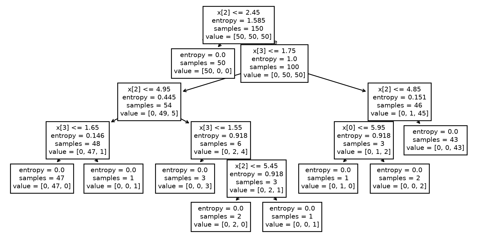
tree.plot_tree(clf)
plt.show()

Example: Visualizing the tree (2/2)

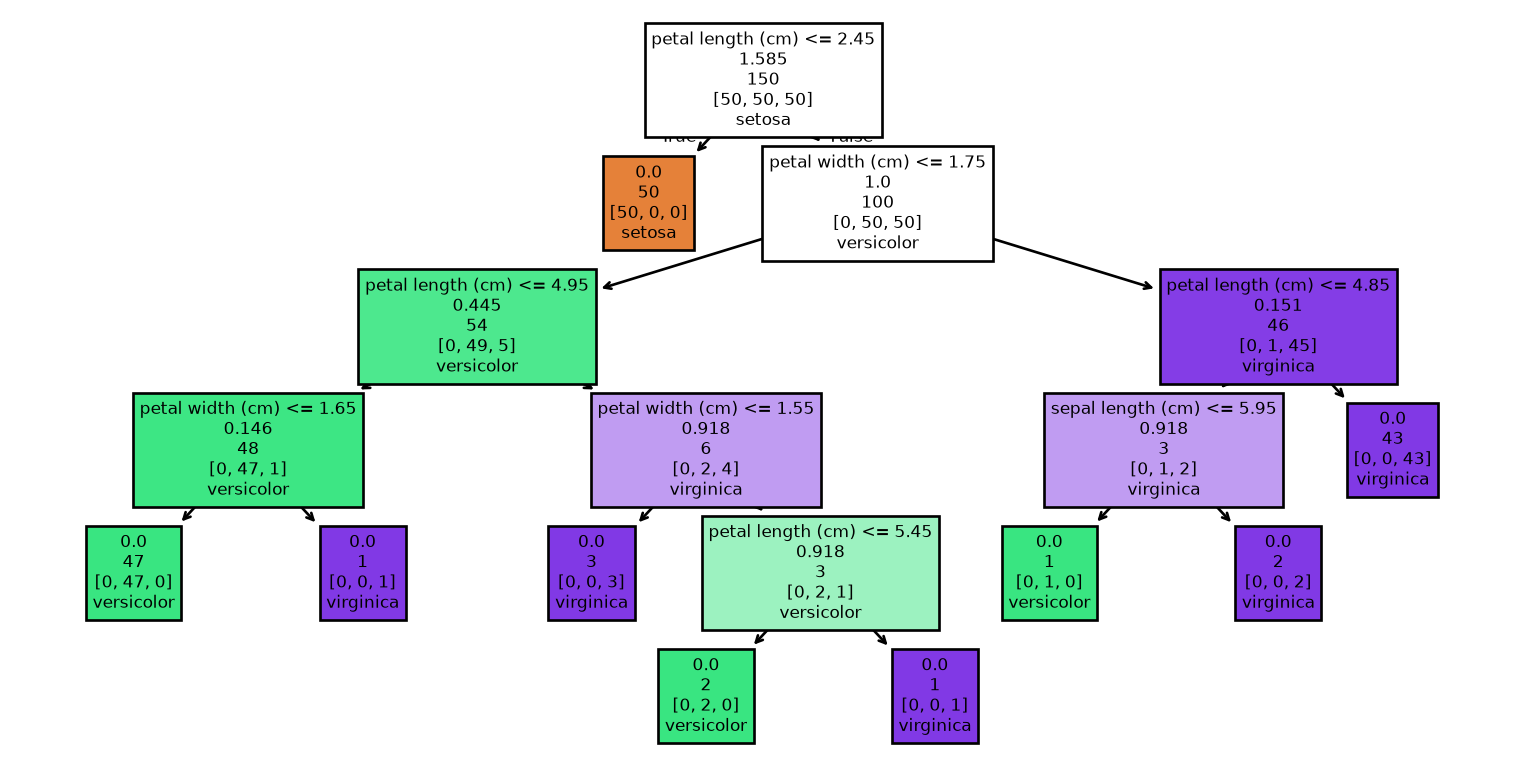
tree.plot_tree(clf, 
               feature_names=iris.feature_names, 
               class_names=iris.target_names,
               label='none',
               filled=True)
plt.show()

In a DecisionTreeClassifier, each internal node of the tree represents a decision based on a feature, each branch represents the outcome of that decision, and each leaf node represents a class label. The decision tree makes predictions by traversing from the root to a leaf node, following the decision rules defined at each node. Decision trees are intuitive and easy to interpret but can be prone to overfitting if not properly regulated.

To build a decision tree, the method fit follows these steps:

1. Evaluate Candidate Splits: For each numerical feature, consider thresholds between observed values.
2. Select the Best Split: Retain the feature and threshold that produce the lowest weighted entropy.
3. Split the Dataset: Send examples to the left or right child according to the selected threshold.
4. Repeat Recursively: Apply the same process within each child. A numerical feature may be used again farther down the tree.
5. Stop Conditions: Stop the recursion when one of the following conditions is met:
   • All instances in a subset belong to the same class.
   • No candidate split improves the objective.
   • A predefined depth limit or minimum number of instances per node is reached.
6. Assign Labels: For each leaf node, assign a class label based on the majority class of instances in that subset.

This process results in a tree where each path from the root to a leaf represents a classification rule.

In the figure above, the decision nodes contain the following information. - The decision rule, e.g. petal width (cm) <= 0.8 - The entropy of the node. - The number of examples in the subset corresponding to this node of the tree. - The number of examples for each of the classes, in the subset corresponding to this node of the tree. - A prediction.

Decision trees are constructed by incrementally adding decision nodes, guided by labelled training examples. A useful split need not separate every class perfectly; it should reduce the weighted entropy of the resulting children. For instance, petal width (cm) <= 0.8 separates Setosa from the other two species in this dataset. When the condition holds (left child), all examples are Setosa. The right child contains Versicolor and Virginica, but no Setosa.

See: - Kingsford and Salzberg (2008), you can access the paper here, html or PDF, from a computer with a uOttawa IP address.

Example: Prediction

# Create two new examples
# 'sepal length (cm)', 'sepal width (cm)', 'petal length (cm)', 'petal width (cm)'

new_irises = [[5.1, 3.5, 1.4, 0.2], [6.7, 3.0, 5.2, 2.3]]

# Prediction

predictions = clf.predict(new_irises)

# Printing the predicted labels for our two examples

print(iris.target_names[predictions])

['setosa' 'virginica']

Example: Complete

iris = load_iris()
clf = tree.DecisionTreeClassifier(criterion="entropy", random_state=42)
X, y = iris.data, iris.target
clf = clf.fit(X, y)
tree.plot_tree(clf)
new_irises = [[5.1, 3.5, 1.4, 0.2], [6.7, 3.0, 5.2, 2.3]]
predictions = clf.predict(new_irises)
print(iris.target_names[predictions])

['setosa' 'virginica']

Example: Performance

from sklearn.metrics import classification_report, accuracy_score

# Make predictions

y_pred = clf.predict(X)

# Evaluate the model

accuracy = accuracy_score(y, y_pred)
report = classification_report(y, y_pred, target_names=iris.target_names)

print(f'Accuracy: {accuracy:.2f}')
print('Classification Report:')
print(report)

The performance of this classifier appears to be perfect at first glance. However, is it really?

Example: Performance

Accuracy: 1.00
Classification Report:
              precision    recall  f1-score   support

      setosa       1.00      1.00      1.00        50
  versicolor       1.00      1.00      1.00        50
   virginica       1.00      1.00      1.00        50

    accuracy                           1.00       150
   macro avg       1.00      1.00      1.00       150
weighted avg       1.00      1.00      1.00       150

Example: Discussion

We have demonstrated a complete example:

• Loading the data
• Selecting a classifier
• Training the model
• Visualizing the model
• Making a prediction

However, several simplifications were made throughout this process.

Example: Take 2

from sklearn.metrics import classification_report, accuracy_score

# Make predictions

y_pred = clf.predict(X)

# Evaluate the model

accuracy = accuracy_score(y, y_pred)
report = classification_report(y, y_pred, target_names=iris.target_names)

print(f'Accuracy: {accuracy:.2f}')
print('Classification Report:')
print(report)

Important

This example is misleading, or even flawed!

The performance of this classifier appears to be perfect at first glance. However, is it really?

Example: Exploration

print(f'Dataset Description:\n{iris["DESCR"]}\n')

Dataset Description:
.. _iris_dataset:

Iris plants dataset
--------------------

**Data Set Characteristics:**

:Number of Instances: 150 (50 in each of three classes)
:Number of Attributes: 4 numeric, predictive attributes and the class
:Attribute Information:
    - sepal length in cm
    - sepal width in cm
    - petal length in cm
    - petal width in cm
    - class:
            - Iris-Setosa
            - Iris-Versicolour
            - Iris-Virginica

:Summary Statistics:

============== ==== ==== ======= ===== ====================
                Min  Max   Mean    SD   Class Correlation
============== ==== ==== ======= ===== ====================
sepal length:   4.3  7.9   5.84   0.83    0.7826
sepal width:    2.0  4.4   3.05   0.43   -0.4194
petal length:   1.0  6.9   3.76   1.76    0.9490  (high!)
petal width:    0.1  2.5   1.20   0.76    0.9565  (high!)
============== ==== ==== ======= ===== ====================

:Missing Attribute Values: None
:Class Distribution: 33.3% for each of 3 classes.
:Creator: R.A. Fisher
:Donor: Michael Marshall (MARSHALL%PLU@io.arc.nasa.gov)
:Date: July, 1988

The famous Iris database, first used by Sir R.A. Fisher. The dataset is taken
from Fisher's paper. Note that it's the same as in R, but not as in the UCI
Machine Learning Repository, which has two wrong data points.

This is perhaps the best known database to be found in the
pattern recognition literature.  Fisher's paper is a classic in the field and
is referenced frequently to this day.  (See Duda & Hart, for example.)  The
data set contains 3 classes of 50 instances each, where each class refers to a
type of iris plant.  One class is linearly separable from the other 2; the
latter are NOT linearly separable from each other.

.. dropdown:: References

  - Fisher, R.A. "The use of multiple measurements in taxonomic problems"
    Annual Eugenics, 7, Part II, 179-188 (1936); also in "Contributions to
    Mathematical Statistics" (John Wiley, NY, 1950).
  - Duda, R.O., & Hart, P.E. (1973) Pattern Classification and Scene Analysis.
    (Q327.D83) John Wiley & Sons.  ISBN 0-471-22361-1.  See page 218.
  - Dasarathy, B.V. (1980) "Nosing Around the Neighborhood: A New System
    Structure and Classification Rule for Recognition in Partially Exposed
    Environments".  IEEE Transactions on Pattern Analysis and Machine
    Intelligence, Vol. PAMI-2, No. 1, 67-71.
  - Gates, G.W. (1972) "The Reduced Nearest Neighbor Rule".  IEEE Transactions
    on Information Theory, May 1972, 431-433.
  - See also: 1988 MLC Proceedings, 54-64.  Cheeseman et al"s AUTOCLASS II
    conceptual clustering system finds 3 classes in the data.
  - Many, many more ...

Example: Exploration

print(f'Feature Names: {iris.feature_names}')

Feature Names: ['sepal length (cm)', 'sepal width (cm)', 'petal length (cm)', 'petal width (cm)']

print(f'Target Names: {iris.target_names}')

Target Names: ['setosa' 'versicolor' 'virginica']

print(f'Data Shape: {iris.data.shape}')

Data Shape: (150, 4)

print(f'Target Shape: {iris.target.shape}')

Target Shape: (150,)

Example: Using Pandas (continued)

import pandas as pd

# Create a DataFrame

df = pd.DataFrame(iris.data, columns=iris.feature_names)
df['species'] = iris.target_names[iris.target]

Example: Using Pandas (continued)

# Display the first few rows of the DataFrame

print(df.head())

   sepal length (cm)  sepal width (cm)  petal length (cm)  petal width (cm)  \
0                5.1               3.5                1.4               0.2   
1                4.9               3.0                1.4               0.2   
2                4.7               3.2                1.3               0.2   
3                4.6               3.1                1.5               0.2   
4                5.0               3.6                1.4               0.2   

  species  
0  setosa  
1  setosa  
2  setosa  
3  setosa  
4  setosa  

Example: Using Pandas (continued)

# Summary statistics

print(df.describe())

       sepal length (cm)  sepal width (cm)  petal length (cm)  \
count         150.000000        150.000000         150.000000   
mean            5.843333          3.057333           3.758000   
std             0.828066          0.435866           1.765298   
min             4.300000          2.000000           1.000000   
25%             5.100000          2.800000           1.600000   
50%             5.800000          3.000000           4.350000   
75%             6.400000          3.300000           5.100000   
max             7.900000          4.400000           6.900000   

       petal width (cm)  
count        150.000000  
mean           1.199333  
std            0.762238  
min            0.100000  
25%            0.300000  
50%            1.300000  
75%            1.800000  
max            2.500000  

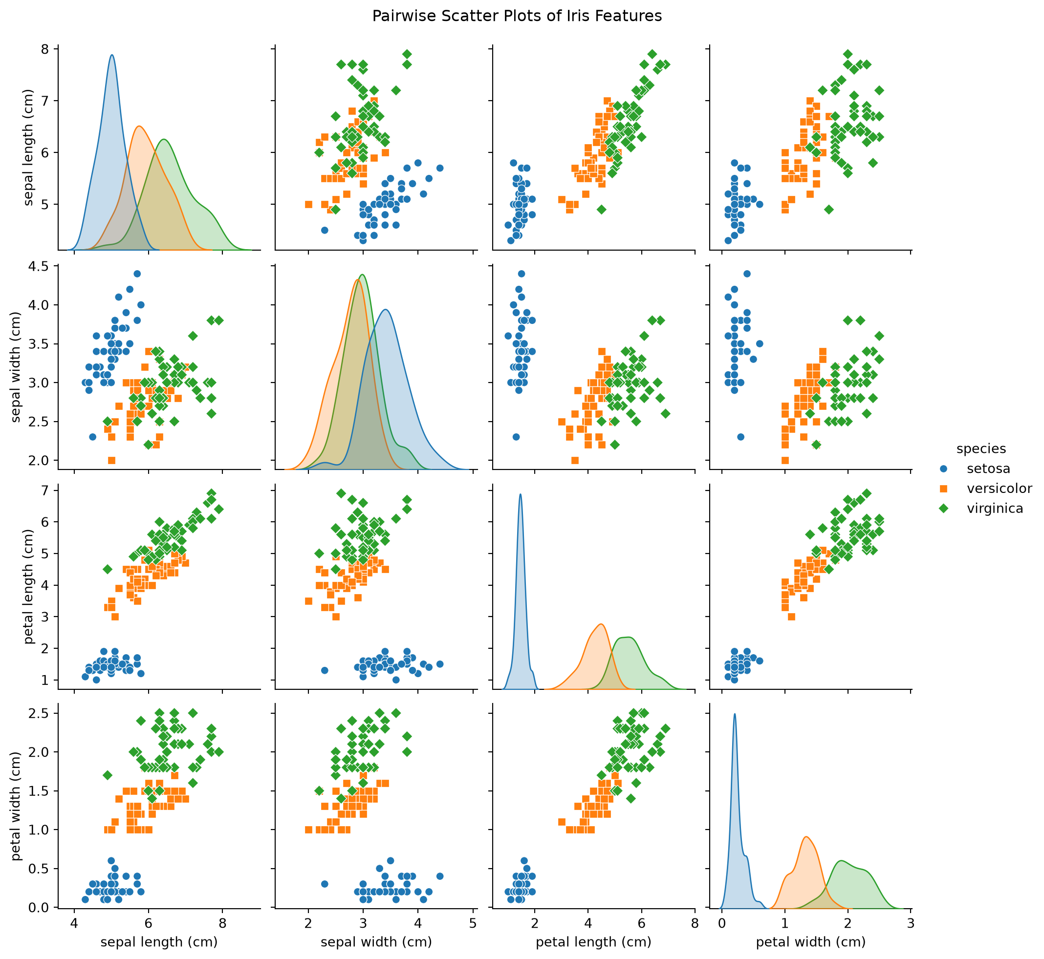
Example: Using Seaborn

import seaborn as sns

# Pairplot using seaborn

sns.pairplot(df, hue='species', markers=["o", "s", "D"])
plt.suptitle("Pairwise Scatter Plots of Iris Features", y=1.02)
plt.show()

What insights can be drawn from examining the graphs?

The figure presents pairwise plots of the Iris features, with the diagonal showing the distribution of each individual feature. Each dot represents an example (x), and the colours indicate its label (y).

Let’s first consider the diagonal elements:

• Is it possible to classify the examples using a single feature?
• We observe that sepal length or width alone cannot distinguish between the classes.
• However, petal length and petal width allow us to distinguish setosa from the other two species, although they do not separate versicolor and virginica perfectly.

The class setosa frequently forms a distinct cluster.

Example: Using Seaborn

Example: Training and Test Set

from sklearn.model_selection import train_test_split

# Split the dataset into training and testing sets

X_train, X_test, y_train, y_test = train_test_split(
    X,
    y,
    test_size=0.2,
    random_state=7,
    stratify=y,
)

We will have a lot more to say about testing in the coming weeks.

For narrative clarity, this appendix explores the full dataset before introducing the split. In a rigorous experiment, the test set should be set aside before making data-driven modelling choices and left untouched until final evaluation.

random_state makes the pseudo-random partition reproducible. Changing it changes which examples are held out and may change the measured accuracy. stratify=y keeps the class proportions approximately consistent across the two subsets.

Practice: Experiment with different values for random_state. What do you observe, and why?

Our initial decision tree was constructed and evaluated using the entire dataset. It can fit those examples closely, but this does not tell us how accurately it will predict unseen data.

Example: Creating a New Classifier

clf = tree.DecisionTreeClassifier(criterion="entropy", random_state=42)

Example: Training the New Classifier

# Train the model
clf.fit(X_train, y_train)

Example: Making Predictions

# Make predictions
y_pred = clf.predict(X_test)

Example: Measuring the Performance

from sklearn.metrics import classification_report, accuracy_score
# Make predictions

# Evaluate the model
accuracy = accuracy_score(y_test, y_pred)
report = classification_report(
    y_test,
    y_pred,
    labels=clf.classes_,
    target_names=iris.target_names[clf.classes_],
)

print(f'Accuracy: {accuracy:.2f}')
print('Classification Report:')
print(report)

Here is a discussion on model persistence for scikit-learn models.

Example: Measuring the Performance

Accuracy: 0.93
Classification Report:
              precision    recall  f1-score   support

      setosa       1.00      1.00      1.00        10
  versicolor       0.90      0.90      0.90        10
   virginica       0.90      0.90      0.90        10

    accuracy                           0.93        30
   macro avg       0.93      0.93      0.93        30
weighted avg       0.93      0.93      0.93        30

Marcel Turcotte

Marcel.Turcotte@uOttawa.ca

School of Electrical Engineering and Computer Science (EECS)

University of Ottawa